Climate Science Glossary

Term Lookup

Enter a term in the search box to find its definition.

Settings

Use the controls in the far right panel to increase or decrease the number of terms automatically displayed (or to completely turn that feature off).

Term Lookup

Settings


All IPCC definitions taken from Climate Change 2007: The Physical Science Basis. Working Group I Contribution to the Fourth Assessment Report of the Intergovernmental Panel on Climate Change, Annex I, Glossary, pp. 941-954. Cambridge University Press.

Home Arguments Software Resources Comments The Consensus Project Translations About Support

Twitter Facebook YouTube Mastodon MeWe

RSS Posts RSS Comments Email Subscribe


Climate's changed before
It's the sun
It's not bad
There is no consensus
It's cooling
Models are unreliable
Temp record is unreliable
Animals and plants can adapt
It hasn't warmed since 1998
Antarctica is gaining ice
View All Arguments...


Username
Password
New? Register here
Forgot your password?

Latest Posts

Archives

Lessons from Past Predictions: Hansen 1981

Posted on 3 May 2012 by dana1981

In previous Lessons from Past Predictions entries we examined Hansen et al.'s 1988 global warming projections (here and here).  However, James Hansen was also the lead author on a previous study from the NASA Goddard Institute for Space Studies (GISS) projecting global warming in 1981, which readers may have surmised from my SkS ID, is as old as I am.  This ancient projection was made back when climate science and global climate models were still in their relative infancy, and before global warming had really begun to kick in (Figure 1).

gistemp to 1981

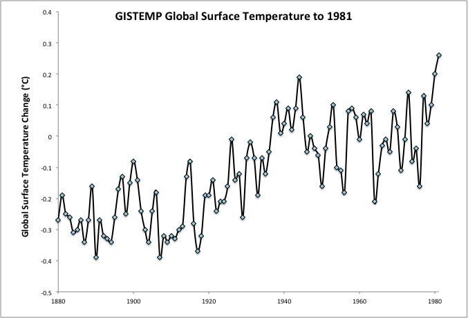
Figure 1: Annual global average surface temperatures from the current NASA GISS record through 1981

As Hansen et al. described it,

"The global temperature rose by 0.2°C between the middle 1960's and 1980, yielding a warming of 0.4°C in the past century.  This temperature increase is consistent with the calculated greenhouse effect due to measured increases of atmospheric carbon dioxide. Variations of volcanic aerosols and possibly solar luminosity appear to be primary causes of observed fluctuations about the mean trend of increasing temperature. It is shown that the anthropogenic carbon dioxide warming should emerge from the noise level of natural climate variability by the end of the century, and there is a high probability of warming in the 1980's."

This analysis from Hansen et al. (1981) shows a good understanding of the major climate drivers, even 31 years ago.  The study was also correct in predicting warming during the remainder of the 1980s.  The Skeptical Science Temperature Trend Calculator reveals that the trend from 1981 to 1990 was 0.09 +/- 0.35°C per decade - not statistically significant because this is such a short timeframe, but most likely a global warming trend nonetheless.

Global Warming Skeptics Stuck in 1981?

Hansen et al. noted that the human-caused global warming theory had difficulty gaining traction because of the mid-century cooling, which ironically is an argument still used three decades later to dispute the theory:

"The major difficulty in accepting this theory has been the absence of observed warming coincident with the historic CO2 increase. In fact, the temperature in the Northern Hemisphere decreased by about 0.5°C between 1940 and 1970, a time of rapid CO2 buildup."

However, as we will see in this post, despite these doubts, the global warming projections in Hansen et al. (1981), based on the human-caused global warming theory, were uncannily accurate.

Climate Sensitivity

Hansen et al. discussed the range of climate sensitivity (the amount of global surface warming that will result in response to doubled atmospheric CO2 concentrations, including feedbacks):

"The most sophisticated models suggest a mean warming of 2° to 3.5°C for doubling of the CO2 concentration from 300 to 600 ppm"

This is quite similar to the likely range of climate sensitivity based on current research, of 2 to 4.5°C for doubled CO2.  Hansen et al. took the most basic aspects of the climate model and found that a doubling of CO2 alone would lead to 1.2°C global surface warming (a result which still holds true today).

"Model 1 has fixed absolute humidity, a fixed lapse rate of 6.5°C km-1 in the convective region, fixed cloud altitude, and no snow/ice albedo feedback or vegetation albedo feedback. The increase of equilibrium surface temperature for doubled atmospheric CO2 is ?Ts ~1.2°C. This case is of special interest because it is the purely radiative-convective result, with no feedback effects."

They then added more complexity to the model to determine the feedbacks of various effects in response to that CO2-caused warming.

"Model 2 has fixed relative humidity, but is otherwise the same as model 1.  The resulting ?T, for doubled CO2 is ~1.9°C. Thus the increasing water vapor with higher temperature provides a feedback factor of ~1.6."

"Model 3 has a moist adiabatic lapse rate in the convective region rather than a fixed lapse rate. This causes the equilibrium surface temperature to be less sensitive to radiative perturbations, and ?T ~1.4°C for doubled CO2."

"Model 4 has the clouds at fixed temperature levels, and thus they move to a higher altitude as the temperature increases. This yields ?T ~2.8°C for doubled CO2, compared to 1.9°C for fixed cloud altitude. The sensitivity increases because the outgoing thermal radiation from cloudy regions is defined by the fixed cloud temperature, requiring greater adjustment by the ground and lower atmosphere for outgoing radiation to balance absorbed solar radiation."

"Models 5 and 6 illustrate snow/ice and vegetation albedo feedbacks.  Both feedbacks increase model sensitivity, since increased temperature decreases ground albedo and increases absorption of solar radiation."

Overall Hansen et al. used a one-dimensional model with a 2.8°C climate sensitivity in this study.  In today's climate models, water vapor is generally a stronger feedback than modeled by Hansen et al. (i.e. see Dessler et al. 2008) and clouds generally weaker (i.e. see Dessler 2010), but their overall model sensitivity was very close to today's best estimate of 3°C for doubled CO2.

Natural Temperature Influences

Hansen et al. discussed the effects of solar and volcanic activity on temperatures, which are the two main natural influences on global surface temperature changes.  Solar activity in particular posed a difficult challenge for climate modelers three decades ago, because it had not been precisely measured.

"for small changes of solar luminosity, a change of 0.3 percent would modify the equilibrium global mean temperature by 0.5°C, which is as large as the equilibrium warming for the cumulative increase of atmospheric CO2 from 1880 to 1980. Solar luminosity variations of a few tenths of 1 percent could not be reliably measured with the techniques available during the past century, and thus are a possible cause of part of the climate variability in that period."

"Based on model calculations, stratospheric aerosols that persist for 1 to 3 years after large volcanic eruptions can cause substantial cooling of surface air...Temporal variability of stratospheric aerosols due to volcanic eruptions appears to have been responsible for a large part of the observed climate change during the past century"

The study compared the various potential global temperature influences of both natural and human effects in Figure 2 below.

Hansen 1981 Fig 2

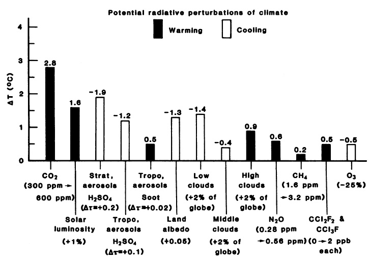
Figure 2: Surface temperature effect of various global radiative perturbations, based on the one-dimensional model used in Hansen et al. Aerosols have the The ?T for stratospheric aerosols is representative of a very large volcanic eruption.  From Hansen et al. (1981)

Hansen et al. ran their model using combinations of the three main effects on global temperatures (CO2, solar, and volcanic), and concluded:

"The general agreement between modeled and observed temperature trends strongly suggests that CO2 and volcanic aerosols are responsible for much of the global temperature variation in the past century."

Due to the uncertainty regarding solar activity changes, they may have somewhat underestimated the solar contribution (Figure 3), but nevertheless achieved a good model fit to the observed temperature changes over the previous century.

100-150

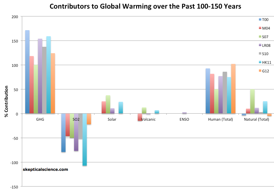
Figure 3: Percent contributions of various effects to the observed global surface warming over the past 100-150 years according to Tett et al. 2000 (T00, dark blue), Meehl et al. 2004 (M04, red), Stone et al. 2007 (S07, green), Lean and Rind 2008 (LR08, purple), Stott et al. 2010 (S10, gray), Huber and Knutti 2011 (HR11, light blue), and Gillett et al. 2012 (G12, orange).

Projected Global Warming

Now we arrive at the big question - how well did Hansen et al. project the ensuing global warming?  Evaluating the accuracy of the projections is something of a challenge, because Hansen et al. used scenarios based on energy growth, but did not provide the associated atmospheric CO2 concentrations resulting as a consequence of that energy growth.  Nevertheless, we can compare their modeled energy growth scenarios to actual energy growth figures.

Figure 4 shows the projected warming based on various energy growth scenarios.  The fast scenario assumes 4% annual growth in global energy consumption from 1980 to 2020, and 3% per year overall from 1980 through 2100.  The slow scenario assumed a growth of annual global energy rates half as rapid as in the fast growth scenario (2% annual growth from 1980 to 2020).  Hansen et al. also modeled various scenarios involving fossil fuel replacement starting in 2000 and in 2020.

Hansen 1981 Fig 6

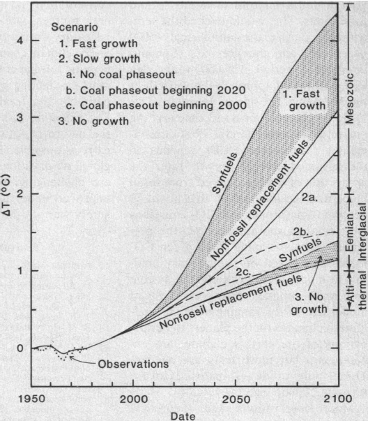
Figure 4:  Hansen et al. (1981) projections of global temperature.  The diffusion coefficient beneath the ocean mixed layer is 1.2 cm2 per second, as required for best fit of the model and observations for the period 1880 to 1978. Estimated global mean warming in earlier warm periods is indicated on the right.

Since 1981, global fossil fuel energy consumption has increased at a rate of approximately 3% per year, falling between the Hansen et al. fast and slow growth scenarios.  Thus we have plotted both and compared them to the observed global surface temperatures from GISTEMP (Figure 5).

Hansen 1981 projections vs observations

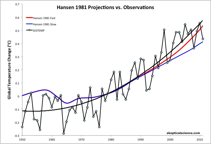
Figure 5: Hansen et al. (1981) global warming projections under a scenario of high energy growth (4% per year from 1980 to 2020) (red) and slow energy growth (2% per year from 1980 to 2020) (blue) vs. observations from GISTEMP with a 2nd-order polynomial fit (black).  Actual energy growth has been between the two Hansen scenarios at approximately 3% per year.  Baseline is 1971-1991.

The global surface temperature record has improved since 1981, at which time the warming from 1950 to 1981 had been underestimated.  Thus Figure 5 uses a baseline of 1971 to 1991 (sets the average temperature anomaly between 1971 and 1991 at zero), because we are most interested in how well the model projected the warming since 1981.  As the figure shows, the model accuracy has been very impressive.

The linear warming trends from 1981 through 2011 are approximtely 0.17°C per decade for Hansen's Fast Growth scenario, 0.13°C per decade for the Slow Growth scenario, vs. 0.17°C per decade for the observed global surface temperature from GISTEMP.  Estimating that the actual energy growth and greenhouse gas emissions have fallen between the Fast and Slow Growth scenarios, the observed temperature change has been approximately 15% faster than the projections of the Hansen et al. model. 

If the model-data discrepancy were due solely to the model climate sensitivity being too low, it would suggest a real-world climate sensitivity of approximately 3.2°C for doubled CO2, although there are other factors to consider, such as human aerosol emissions, which are not accounted for in the Hansen et al. model, and the fact that we don't know the exact atmospheric greenhouse gas concentrations associated with their energy growth scenarios.

Predicted Climate Impacts

Hansen et al. also discussed several climate impacts which would result as consequences of their projected global warming:

"Potential effects on climate in the 21st century include the creation of drought-prone regions in North America and central Asia as part of a shifting of climatic zones, erosion of the West Antarctic ice sheet with a consequent worldwide rise in sea level, and opening of the fabled Northwest Passage."

We can check off all of these predictions. 

Christy's Poor Critique

Climate "skeptic" John Christy, whose poor analysis of Hansen et al. (1988) we previously discussed, has also recently conducted a poor analysis of Hansen et al. (1981), posted on Pielke Sr.'s blog.  Christy attempts to compare the warming projections of Hansen et al. with his lower atmosphere temperature record from the University of Alabama at Huntsville (UAH).  However, Christy is comparing modeled surface temperatures to lower atmosphere temperature measurements; this is not an apples-to-apples comparison.

Christy's justification for this comparison is that surface temperature records and UAH show a similar rate of warming over the past several decades, but according to climate models, the lower atmosphere should warm approximately 20% faster than the surface.  Christy believes the discrepancy is due to a bias in the surface temperature record, but on the contrary, the surface temperature record's accuracy has been confirmed time and time again (i.e. Peterson et al. 2003, Menne et al. 2010, Fall et al. 2011 [which includes Anthony Watts as a co-author!], Muller et al. 2011 [the BEST project], etc.).  There are good reasons to believe the discrepancy is primarily due to problems in the atmospheric temperature record, but regardless, a surface temperature projection should be compared to surface temperature data.

In addition, Christy removes the influence of volcanic eruptions (which have had a modest net warming effect over the past 30 years due to a couple of volcanic eruptions causing cooling during the early part of that timeframe) before comparing UAH record to the Hansen model projections, but he fails to remove other short-term effects like the El Niño Southern Oscillation (ENSO) and solar activity (as was done by Foster & Rahmstorf [2011]), which have had cooling effects over that period.  As a result, Christy's analysis actually biases the data in the cool direction prior to comparing it to the model, and as a result he arrives at the incorrect conclusion, wrongly claiming that Hansen et al. had over-predicted the ensuing global warming.

From Intrigue to Concern

The concluding paragraph of Hansen et al. expresses fascination at the global experiment we are conducting with the climate:

"The climate change induced by anthropogenic release of CO2 is likely to be the most fascinating global geophysical experiment that man will ever conduct.  The scientific task is to help determine the nature of future climatic effects as early as possible."

While the grand global experiment humans are running with the climate remains a fascinating one, climate scientists have concluded that the nature of future climatic effects will be predominantly bad if we continue on our current greenhouse gas emissions path, and potentially catastrophic.  Over the decades James Hansen's tone has grown increasingly alarmed, as he and most of his fellow climate scientists worry about the consequences of human-caused climate change.

Hansen et al. (1981) demonstrates that we have every reason to be concerned, as three decades ago these climate scientists understood the workings of the global climate well enough to predict the ensuing global warming within approximately 15%, and accurately predict a number of important consequences.  It's high time that we start listening to these climate experts and reduce our greenhouse gas emissions.

0 0

Printable Version  |  Link to this page

Comments

Comments 1 to 46:

  1. Thanks Dana! Fascinating stuff, and I wonder if Hansen in '81 had any inkling as to what lengths some would be prepared to go to keep the 'fascinating global geophysical experiment' running! I've yet to receive a reply to a related question from any self-described 'conservative' contrarian: 'What is the conservative position on conducting a radical experiment with the one atmosphere we possess?' I'm surprised this post has been up for so long without receiving flak, given it's about Hansen's projections, which are second only to the hockey stick, surely, as a target of 'skeptic' ire! But no doubt it's coming...
    0 0
  2. Dana, Good job. It is remarkable how accurate this paper was. As you show, it is difficult now, 30 years later, to determine if Hanasen was right on with his prediction or slightly low. Realclimate recently posted a similar analysis of Hansen 1981. They have similar conclusions to yours. Of course we will get skeptics (on other threads) claiming Climate Theory does not make predictions that can be falsified! Link them to this one!
    0 0
  3. I looked at this paper myself after Hansen's TED talk and featured it on my own blog; What Hansen et al got right decades ago. http://reallysciency.blogspot.co.uk/2012/03/what-hansen-et-al-got-right-decades-ago.html
    0 0
  4. I hope you'll know I'm not being 'skeptic', in the climate sense of that word, but I am a bit confused. This appears to be saying that Hansen's 1981 work is good because it made a reasonably accurate prediction. But the previous take on his later 1988 work doesn't make sense to me: "Hansen's 1988 projections were too high mainly because the climate sensitivity in his climate model was high. But his results are evidence that the actual climate sensitivity is about 3°C for a doubling of atmospheric CO2." So I don't really know what's being said. If predictive success is the criteria, didn't Hansen get something wrong in the later work? If so, what changed? If, as I think the 1988 analysis is saying, the point is rather that Hansen's model structure was correct, but he just got some parameter values a bit skewy, *why* were they skewy? How did his work make worse predictions later? Don't we want predictive success to be the criteria for climate models, and shouldn't that include asking how incorrect sensitivity estimates were arrived at? I'm imagining the answers are in the papers somewhere, based on what kind of modelling each was doing, so apologies - this is just a first-glance reaction.
    0 0
  5. @Dan #4 Mine is a layman's comment; but the way I've always thought of model predictions is not -- as fake sceptics like to portray them -- scientific fortune telling where success is measured on how close they prove to be to reality; but rather as useful indicators, which might or might not work out depending on whether the parameters that they are built on, change. It's therefore possible for a model prediction to 'get lucky' -- like picking the Derby winner -- but not technically be as useful as another model where a base parameter changed after publishing but the model usefully predicted what could have happened. I guess what I'm saying is that it's probably best not to trumpet the 'success' of models that happen to 'get lucky' because it then makes it more difficult to defend models that didn't. The truth is, 'right' or 'wrong', they're all useful in their own way. Have I got this right?
    0 0
  6. John #5: that's a plausible explanation for me, if it's right, and does fit with what Dana appears to have said. That is: the model structure was good in 81. Calibration later provided better sensitivity estimates. That still leaves me wondering why the model method's skill seemed to get worse in the intervening years (or wondering if an entirely new modelling approach was used... I should read the papers, shouldn't I!?) I take your point on getting lucky: precisely why testing through straightforward data-fitting is always a bit tricksy. But if sensitivity estimates improved in the intervening years, I'd have expected the model range to become more accurate too. The problem's at least in part that the 81 model doesn't appear to supply any range/s.d. values - maybe the full paper does?
    0 0
  7. Dan Olner - the overall difference is that the sensitivity of the model used in 1981 was 2.8°C while the sensitivity of the model he used in 1988 was 4.2°C. Evidence now indicates that the sensitivity of the '81 model was quite close to the real-world. As to why the sensitivity of the earlier model was closer to the real-world value, that's a difficult question to answer, because model sensitivity is a result of the many different complex parameters of the model. It probably has something to do with the representations of the oceans and ocean processes, which are very difficult to model, as I understand it. But that's a question for a modeling expert, which I am not. Regardless, the bottom line is that both model projections suggest that real-world sensitivity is close to 3°C for doubled CO2. The most interesting aspect of these old model projections is not whether they were "right," but what we can learn from them.
    0 0
  8. Dan Olner (and dana1981): There is a really big difference between the 1981 and 1988 papers in terms of the type of models. The 1981 paper used a one-dimensional radiative-convective model, which resolves the vertical atmosphere and detailed radiation transfer very well, but has no "geography" - it simulates a global average condition, and the primary output is a single temperature profile. The 1988 paper used a 3-d general circulation model. Completely different beasts. It's not a matter of the 1988 work being a tweaking or adjustment of the 1981 model - it's a major change in the analysis. In 1981, a radiative-convective model (RCM) would have been well-developed, and the success in getting a sensitivity close to today's "best estimate" is [you choose] a) somewhat fortuitous, or b) an indication that even a 1-d model of this type can represent many of the important factors. You don't see much use of RCMs these days, when it comes to trying to narrow down sensitivity - they don't do the things that need to be examined. In 1988, GCMs were still undergoing significant development - as they are today, muchly due to greatly increased computing power. GCMs are hungry beasts, and eat CPU cycles like Chiclets. Everyone on the team likely wants some extra FPU time, and a faster computer will always let you do more stuff that was only a gleam in the eye last year. In 1981, Hansen et al wouldn't have had the horsepower to run a GCM (they did exist) over a time period like they did with the RCM.
    0 0
  9. "ancient projection"? 1981 wasn't that long ago, you whipper snapper! :-)
    0 0
  10. #7 dana1981 - Equilibrium climate sensitivity is usually measured in GCMs by incorporating a 'slab ocean' - i.e. an 'ocean' which is little more than a surface with a low heat capacity. This is done because fully equilibrating a GCM with a realistic model of the ocean can take several centuries to millennia due to thermal inertia, and that means a large computation expense. Point being, representation of oceans can't have much effect on ECS, as traditonally measured.
    0 0
  11. John: "ancient", when it comes to age, generally tends to follow the rule that anyone older than 10*(my age)^0.5 is "ancient". For the young whipper-snapper who is 30-31, square root of that times 10 is about 55, so I am ancient by his standards, as I just turned 55. When he was 16, 40-year-olds seemed "ancient" - and I would have been 40, so I was ancient to him back then, too. As I am old enough to remember discussing Hansen et al, 1981, in grad school, I must be really ancient. [By the time you get to be 100, you are ancient.]
    0 0
  12. pauls: Do you have a reference showing that a "GCM with a realistic model of the ocean" is run in a mode where it only uses a slab ocean that is "little more than a surface with a low heat capacity"? Such "swamp models" were very common in the early days of GCMs (i.e., back in the 1960s and 1970s - remember: I'm "ancient") due to computational issues, but I can't see how it would be of any use to develop a fully-coupled atmosphere-ocean GCM to investigate how climate reacts when full ocean dynamics are included, and then shut off the ocean dynamics to investigate the long-term sensitivity. In other words, my hunch is that you're wrong, but my mind is open to whatever references and evidence you can provide.
    0 0
  13. Bob Loblaw, IPCC chapter 8. Check the caption for table 8.2.
    0 0
  14. pauls: Thanks. I'll try to read through it. I'll also be off the net for the next week or so, so I won't be able to reply soon.
    0 0
  15. pauls: I've actually had a chance for a quick look at the IPCC section you linked to. Please refer to the section of text in Section 8.6.2, and note the part where is says:
    and is often simply termed the ‘climate sensitivity’. It has long been estimated from numerical experiments in which an AGCM is coupled to a simple non-dynamic model of the upper ocean with prescribed ocean heat transports (usually referred to as ‘mixed-layer’ or ‘slab’ ocean models) and the atmospheric CO2 concentration is doubled.
    You referred in your comment to the "slab ocean", and called it "little more than a surface with a low heat capacity". In contrast, the IPCC report talks about the mixed layer (roughly 60-100m thick) of the ocean, and specifically says that it has "prescribed ocean heat transports". That doesn't sound like "a surface with a low heat capacity" to me. It sounds like they are leaving out the deep ocean, not calculating ocean movements, but just specifying the heat storage and transfer within the mixed layer. Can you explain why you think this is "just a surface with a low heat capacity"? I will continue to look through the IPCC report, to see if there are more details. It may be necessary to look at some of the papers in its references, however. I'd like to know more about just what "ocean heat transports" are prescribed.
    0 0
  16. Bob Loblaw, I've found a nice, simple description of slab-ocean models: http://www.boinc-wiki.info/Slab_Model The ocean heat transports are the currents moving heat around the planet. Prescribing them means the model doesn't have to calculate dynamically, another reason ocean modelling doesn't have much influence on measured ECS on GCMs. The point I'm making about the shallowness of the slab-ocean is this: 'As the ocean is simplified it does not take a long time for the ocean to fully adjust to the new forcings and therefore the climate does not take anywhere near as long to settle down into its final pattern. (Like 20 model years instead of over 200 model years.) You can therefore get a reasonable idea of the overall effect of a forcing like an x% increase in CO2 in a shorter amount of computer time.'
    0 0
  17. Newbie physicist here, not climate guy, trying to understand. Try as I might I cannot figure out which of the models are used in the important Fig. 6 of the seminal 1981 result (Science, 213, pp. 957-966)I have read the paper a lot. Is the "model two" plotted which uses the CO2 temp increase then constrains relative humidity to be constant? Or 5/6 models which have albedo feedback? Apologize for the fact this post duplicates another I made in a less appropriate thread. I teach kind of a "Physics of Environment 101" at a University and am trying to sharpen up.
    0 0
  18. Hi curiousd. I believe Figure 6 is a plot using Model 4, actually. If you look at the top of page 3 of the paper (page 959 in the journal), it says Model 4 has the climate sensitivity they're using of 2.8°C for doubled CO2. Prior to that they note that they didn't have enough knowledge at the time to include the vegetation feedback for Models 5 and 6, so 4 was advanced as they could get with reasonable confidence.
    0 0
  19. Tank you Dana. If you don't mind another question, from other answers to my questions I gather that no matter what the CO2 concentration, doubling the CO2 produces the same change in temperature. I think this means that C2 = C1 x 2^(delta T1/3) if 3 is the "climate sensitivity" as is called in your field. But so far I have not come across this expression. Am I correct here? In other words if delta T = 3 , C2/C1 = 2. If in the future C3/C2 = 2 then C3 = 4C1 so that C3 = C1 x 2^(2 deltaT1/3). In other words, CO2 concentration varies exponentially with temperature change. Do I have this correct?
    0 0
  20. curiousd @18, the standard formulas are: 1) dF= ln(C2/C1)*5.35 2) dT=0.75*dF The margin of error for the first constant is +/- 10%. That for the second is approximately 0.55-1.1 dF is change in forcing in W/m^2, dT is change in temperature in degrees Kelvin, C2 and C1 are as per your definition. Clearly these formulas are simple approximations. In particular, the first formula cannot be valid for very low atmospheric concentrations or else forcing would be infinite. It is, however, approximately accurate for the range of CO2 concentrations that may have been experience on Earth over the last 600,000 years (150-8000 ppmv) and therefore also over the range of CO2 concentrations humans are likely to produce in the atmosphere.
    0 0
  21. Thanks Tom Curtis. Huh! Then Equate the dFs in 1 and 2 You get dT/0.75 = ln(C2/C1)x 5.35 dT / 4.01= ln (C2/C1) e^(dT/4.01)= C2/C1 = 2^ (dT/X) ; set c2/c1 = 2 and what is unknown X? X = 2.8 Then: equivalently (C2/C1) = e ^ (dT/4.01) (C2/C1) = 2 ^ (dT/2.8) By getting rid of the dF you get that (C2/C1) depends exponentially on dT and the formula with the 2 base shows the doubling temperature (climate constant)perhaps more clearly. So.....this way one can get climate constant into the "exponential growth" section of a basic course. And an exponential growth versus time in CO2 yields a linear growth versus time in dT.
    0 0
  22. OOPS! No my last sentence beginning "And" is wrong above. Because the dT contains rapid response components and long response components. I was forgetting about that important point.
    0 0
  23. curiousd @21, I believe your mathematics is correct (though maths is not my strong suite). What is absent is an awareness of the physics. Your formula would be useful to predict the change in CO2 concentration if: a) We used the measured climatology (>29 year mean) of Global Mean Surface Temperature for two periods, commencing t1 and t2 to determine dT; b) t1 and t2 where sufficiently far apart in time for the Earth to reach an equilibrium response to a change in forcing; c) t2 was sufficiently long after the last change in CO2 concentration for the Earth to have reached the equilibrium climate response; and d) Change in CO2 levels where the only change in forcing between t1 and t2. For conditions (b) and (c), a sufficient period is certainly not less than a century, and may be considerably longer. Conditions (a) through (c) when we compare data from paleoclimatology with each other, or to present values. Condition (d) has probably never been satisfied on Earth, and is certainly not being currently satisfied. The standard formulas are useful because we can calculate the change in forcing for a variety of forcings, sum them and then calculate to a first approximation the expected Equilibrium Climate Response. Being more accurate, we would apply a weighting to each forcing separately to allow for the fact that different forcings have slightly different feedback responses due to differences in geographical, vertical and temporal distribution. By definition, the weighting of CO2 = 1. (We could of course, define any other forcing as having a weighting of 1 instead, simply by varying the constant in the second equation.) So, given the above, my question is, where are you going with your equation?
    0 0
  24. curiousd @22, you can partially eliminate that problem, and conditions (b) and (c) in my 23 by calculating the Transient Climate Response, which is about 2/3rds of the ECR (with a large uncertainty). However, the remainder of my points from my 23 would still stand.
    0 0
  25. Hi Tom Curtis, Say you are teaching this stuff to people who are paranoid of even simple algebra, and have been dragged kicking and screaming into a situation where they have to learn some math and physics to graduate. If they are to be tortured by math and physics anyway might as well give them problems like this: From Mona Loa data the annual growth of CO2 in the decade 2000 - 2010 is reasonably constant and averages about 2 ppm/year. The concentration of CO2 in the atmosphere in 2000 was about 360 ppm. (a) If present growth rates of CO2 continue, what is the "doubling time" in years for CO2? Standard rule of thumb for non scientists with math paranoia: D.T. = 70/ % increase. They would struggle to figure out what % increase 2 out of 360 was, but about half the class would do it correctly and get 116 years. (b) Climatologists have a parameter they call the "Climate Sensitivity" which is the temperature increase that is eventually guaranteed for a doubling of CO2. It could perhaps also be called the "doubling temperature." What would the eventual increase expected in world temperature that would result from 232 years of CO2 growth at the rate of the 2000 - 2019 decade? This is two doubling times of growth, which result in two doubling temperatures or an eventual guaranteed increase of 5.6 degrees C I would then ask them to compute the equivalent change in degrees F and here I would get really crazy answers from about half the class which I would need to adjust.
    0 0
  26. Hi again Tom Curtis, I should also say that we do teach - say in talking about multiplying bacteria - that N = N1 x 2^(t/d.t.), d.t. is doubling time (You cannot use the e base with these folks for obvious reasons). But now I can say that there is an analogous expression that applies to something climate scientists call the climate sensitivity and the expression is C= C1 x 2^( T increase eventual/ T climate sensitivity). However - T increase eventual is indeed eventual - there is a fast reacting and slow reacting component. All this gives me a handle to incorporate and connect the climate sensitivity concept into the lecture on exponential growth, population growth, demographic transition, and so on then ask problems like the one I put into post 25.
    0 0
  27. Curiousd, at 2 ppm per year, a 360 ppm starting point, and a 560 ppm target (two times the historical ~280 ppm amount) it would take (560 - 360) / 2 = 100 years (i.e. 2100) to reach double the historical CO2 level. To double again to 1120 ppm it would then take another 280 years if the 2 ppm increase per year held constant. I'm not sure how you are getting the 116 years figure (among other things it seems to assume annual increase remains a constant percentage of the accumulated total... which contradicts your own statement of a 2 ppm constant increase), but even if it were correct it could not then simply be extrapolated to another 116 years to forecast another doubling of CO2 levels as you indicate. If the rate of increase remains constant then the time required to double that atmospheric CO2 level also doubles. All that being said, the rate of atmospheric increase has not been constant. In the 1990s it was a bit below 2 ppm per year and it is now a bit above. However, this rate of acceleration is largely dependent on levels of human fossil fuel use and thus predictions of what it will be a century out are little more than guesswork.
    0 0
  28. Thanks CB.....short of it was that late at night I was misreading a stack of data on CO2. Sorry. One more tho.. Since it turns out that the dF = ln (C2/C1)x const leads to that exponential formula I got, this got me to thinking about where that logarithmic dependence on concentration comes from, since by standard Beer's law physics you would expect an exponential to a power with an effective absorption coefficient involved. I was digging all around the net and I guess maybe this ln dependence is empirical, and has to due with the fact that the CO2 only allows radiation to go through at the wings of the transmission window? If the derivation is really that hairy then for my purposes I don't need to go through it, but just checking here.
    0 0
  29. curiousd, the logarithmic expression for dF in terms of CO2 concentrations is empirically derived from observations and calculations using radiative transfer codes, not established from first principles, and in fact it's only a first-order approximation that is "accurate enough" (given other uncertainties) for the ranges of CO2 concentrations that are of concern to us. As you can see from the TAR, various approximations have been used at different times by different authors, although they're all pretty similar. Because it's logarithmic, an exponential increase in concentration will result in a linear increase in temperature (ignoring feedbacks). Unfortunately, CO2 concentration has been increasing at a rate greater than exponentially so the CO2 forcing is growing faster than linearly.
    0 0
  30. curiousd you can not use Beer's law to calculate the forcing; you can not even use it to calculate the infrared flux to space. You need to take into account the absorbed as well as the emitted fluxes, the vertical profiles and the wavelength dependence. This is what a radiative transfer code does. The simplified formula is just a empirical fit. Here's the paper.
    0 0
  31. Hello All, Curious D back with more questions pertaining to explaining all this to a basic physics class. So.. 1. You folks have taught me that there is a logarithmic dependence of dF in terms of CO2 by empirical results or simulations. Therefore, an exponential growth of CO2 concentration leads to a linear increase in expected T with time. But.. 2. there are separate fast responses and long term responses. Therefore: 3. If by magic, all CO2 going into the atmosphere were to stop, there would still be another shoe (or maybe more than one shoe) to drop. I figured out the predicted temperature increase of Hansen's 1981 paper assuming only his CO2 alone plus the constant humidity water vapor based on his results from his "model one" and I think it gives just about the observed 0.8 degrees C. O.K. BUT 4. The "removing ice decreased albedo" feedback has not really struck home yet from assuming CO2 about 40% increase over pre industrial levels. Correct? Then: 5. Is a 40% increase in CO2 enough to eventually melt Greenland?(i.e. even in a magic world with no more CO2 Greenland ice is eventually toast anyway. Yes? No?) 6. How can there be a constant climate sensitivity, including long term feed backs, if large fractions of the world ice were gone? If there were no ice left would there not be an "as bad as it can get" effect on the climate sensitivity? No ice left means no ice-albedo feedback anymore? (Yes? No?) I am completely on board with the notion that AGW is probably an existential threat exceeding all out nuclear warfare, but for me it is really, really important to have all my ducks in a row when teaching this stuff. So I do not see how the idea of a constant eventual increase in temperature is associated with CO2 doubling if you compare the situation with lots of ice left (now) with no ice left (eventually BAU), because of the "as bad as it can get effect in terms of "ice melting - albedo lessening feedback".
    0 0
  32. More focused statement about what bothers me about understanding how climate sensitivity concept jibes with 1981 model result..what is a fast response, what is a slow one and so on. Here are two answers that were given to my questions about the fact that apparently the concentrations of CO2 C2/C1 = 2^(t/2.8), and then about the 1981 calculation of Hansen. I had asked which of his models were plotted in the graph. 1. Dana 1981: Hi curiousd. I believe Figure 6 is a plot using Model 4, actually. If you look at the top of page 3 of the paper (page 959 in the journal), it says Model 4 has the climate sensitivity they're using of 2.8°C for doubled CO2. Prior to that they note that they didn't have enough knowledge at the time to include the vegetation feedback for Models 5 and 6, so 4 was advanced as they could get with reasonable confidence. 2. Am not sure string for this next comment here but: curiousd @53, across a wide range of CO2 concentrations, including all those that have been experienced on Earth in the last 600,000 years or are projected under anthropogenic emissions, doubling CO2 results in a 2-4 degree increase in temperature if we ignore slow feedbacks such as melting of ice sheets. The IPCC best estimate for that figure is 3 degrees C. But if (second comment) the climate sensitivity of about 3 degrees is not slow feedback, then if CO2 has increased by ~40% since pre industrial levels, doesn't this mean, since by first comment they have climate sensitivity of 2.8 in 1981 graph, that C2/C1=1.4 if 40% increase in CO2 since pre industrial era. But C2/C1 = 2^(t/2.8) should have been observed, t is temperature increase. (Check....at t = 2.8, C2/C1 = 2) So 1.4 = 2^(t/2.8) ; solving t - the temperature increase - would be about 1.3 degrees. But we have only seen about 0.8 degrees. I do think they get the 0.8 degrees for 1981 model that had just CO2 direct effect plus holding relative humidity constant to get a water vapor feedback.But then the "climate sensitivity" is not 2.8 degrees????? This all would make sense to me if that 2.8 degrees climate sensitivity did contain a long term feedback we have not seen yet. But from the second comment, that 2.8 does not include the ice/albedo thing, and should therefore be short term??? But then we should have seen over a degree by now? There is a good possibility I am just being dense about this, I know.
    0 0
  33. CuriousD The temperature anomaly is not the same as the increase in temperature due to GHG forcing. Human activities force the temperature both up and down. Therefore the temperature impact of GHGs = temperature anomaly + temperature impact of sulfates et al.
    0 0
  34. Tristan, I can find no place in the article by Hansen, et al in 1981 that states they include sulfates in their calculations. GHG effects only. And at the same time on many places in this site the fact that the 1981 calculation gets the 0.8 degree C increase right is taken as excellent confirmation of their approach. I don't see how all this agrees with your statement, which is - I guess? - that the observed temperature increase is not expected to agree with a GHG only calculation??
    0 0
  35. O.K. Tristan. Maybe I see it? They normalized their zero point on the graph to 1950, and by the 1940s there had already been a lowering of temperature due to aerosols. So the predicted 0.8% increase was by this kind of normalizing, taking the aerosols into account. So if I am right that 2.8% climate sensitivity would have produces a 1.3% increase with no aerosols, maybe this means that the aerosols we have contribute about half a degree cooling? BTW the sensitivity doubled in their model four when they put into the model that clouds move to a higher altitude as temperature increases. Does this mean we can fight global warming by having vehicles/factories that produce as much of certain kinds of obnoxious smog emissions`as possible? Only partially kidding, here.
    0 0
  36. Curiousd, Geoengineering schemes have been proposed using sulfates to lower surface temperature. The Chinese have started implementing these efforts ;). One side effect of this scheme that is not often mentioned by proponents is that it significantly lowers evaporation from the ocean surface. This causes drought. Sulfates also make ocean acidification worse. Choose your poison: heat or drought. The 3C climate sensitivity is an equilibrium change. You are doing your calculations using only the realized temperature change. The climate is not in equilibrium so you are substantially underestimating the sensitivity. All the observed change so far is from the "fast" feedbacks. These take decades to come to equilibrium. Remember, we are talking about the entire Earth. The slow feedbacks, like melting ice sheets, take decades or centuries to come into play. These are difficult calculations to make. Read more before you make any conclusions based on your own calculations. For myself, I rely on Hansen's papers (and the IPCC) and do not attempt to check the calculations.
    0 0
  37. curiosd - as michael sweet notes @36, the 2.8°C climate sensitivity value is an equilibrium value. That's how much the planet will ultimately warm once it reaches a new energy balance. That takes time because of the heat storage in the oceans. This is called the thermal inertia of the climate system. It takes many decades - even over a century for the new equilibrium state to be reached. What you're looking at is called the transient climate response - how much the planet warms immediately - which is roughly two-thirds of the equilibrium response.
    0 0
  38. CuriousD, Concerning this comment:
    How can there be a constant climate sensitivity, including long term feed backs, if large fractions of the world ice were gone? If there were no ice left would there not be an "as bad as it can get" effect on the climate sensitivity? No ice left means no ice-albedo feedback anymore? (Yes? No?) I am completely on board with the notion that AGW is probably an existential threat exceeding all out nuclear warfare, but for me it is really, really important to have all my ducks in a row when teaching this stuff. So I do not see how the idea of a constant eventual increase in temperature is associated with CO2 doubling if you compare the situation with lots of ice left (now) with no ice left (eventually BAU), because of the "as bad as it can get effect in terms of "ice melting - albedo lessening feedback".
    You seem be making two errors in your general appreciation of the situation. First, you seem to have latched onto the ice-albedo feedback as "the feedback" (possibly because it is something that is very easy to visualize and conceptualize). Second, you seem to think that climate sensitivity is a hard and fast "universal constant." There are many feedbacks in both directions. The feedbacks for any particular configuration (starting temperature, type of forcing, continental and ocean current configurations, etc.) are very, very different. Those parameters affect the exact feedbacks that occur, and that in turn varies the climate sensitivity. No two scenarios have exactly the same climate sensitivity. It's not a simple linear equation. It's an extremely complex, multi-dimensional problem with thousands of variables. There is no way to truly know exactly what the climate sensitivity is in our particular situation... short of running the exact experiment we're running right now, which is to apply a forcing and then see what happens. What we do know is that: 1) Studies of immediate observations point to a climate sensitivity between 2.5˚ to 4˚ C. 2) Studies of models, which attempt to incorporate as many factors as we can, as best we can, point to a climate sensitivity between 2.5˚ to 4˚ C. 3) Studies of many past climates -- admittedly all different from today's, as they all must be -- point to a climate sensitivity between 2.5˚ to 4˚ C. It's never going to be a scenario where you can say "well, ice albedo feedback will do exactly this, and methane feedback will do exactly this, and... it all adds up to exactly this." [As an aside, concerning the Arctic... suppose all of the ice does melt? What about all of the methane that is stored, on land and in the oceans? What temperature change would it take to release that, and how much might be released? Part of the problem here is that one can't necessarily anticipate all of the feedbacks, and properly quantify them. No matter what you think of, you're likely to be in for some rude shocks.]
    0 0
  39. curiousd @34 and 35, on page 958 in the article, Hansen writes:
    "The radiative calculations are made by a method that groups absorption coefficients by strength for efficiency. Pressure- and temperature-dependent absorption coefficients are from line-by-line calculations for H2O, CO2, O3, N2O and CH4, including continuum H2O absorption. Climatological cloud cover and aerosol properties are used ..."
    That means aerosols equivalent to the average over the period of climatology (probably 1951-1980, although I am unsure) where used in the model. This means changes in aerosols after that period are not included in the model, but because of clean air acts in Western Democracies in the 1970s, and the collapse of Eastern European industry with the fall of the Soviet Union and unification of Germany, the increases in aerosols have been small over that period.
    0 0
  40. Hi, Dana and Michael and everyone else here, I am trying to pin this down, that's all. So I understand it. In the 1981 Hansen calculation he used a succession of models and his 2.8 climate sensitivity included (a) CO2 alone (1.2 degrees) (b) water vapor feedback by holding the relative humidity constant (1.9 degrees)(c) something called the moist adiabatic lapse rate - which I have no clue about yet (down to 1.4 degrees) , and "Clouds at fixed temperature levels so they move to higher altitudes as temp increases" (back up to 2.8%) so that 2.8 % does not contain any long term feedbacks!! Elsewhere on this site I have been told that indeed the 2.8 does not contain the long term ice - albedo feedback. The only calculations I am doing is taking the climate sensitivity for the various effects as calculated by Hansen, et all, and plugging into C2/C1 = 2 ^ (t/tsensitivity). What is wrong with that?
    0 0
  41. Hi Sphaerica, Sure, all kinds of surprise effects might come about - like releasing methane from the Arctic....but my motivation here is just to find out: Is the temperature increase, including all effects long and short term, always given by concentration proportional to exponential of the increase? This academic question is of interest to me because my path to do my bit here runs through education and includes being able to explain this stuff accurately to people most of whom have PhDs in physics, but none of whom have much of a clue about climate science. They will think this exponential dependence of the concentration on temperature increase is really neato in a geek like way and quite unexpected, but will ask questions. The first question likely will be: if this relationship includes the effect of the ice albedo, then how can you continue to have the same exponential dependence, in principle, even after the ice is melted? I think the discussion you give in post 38 tells me that "No, the exponential relationship cannot be in principle constant over the very long term with unchanging climate sensitivity." Tom Curtis, Your post was extremely helpful. So in my post 38 all I did was to use the exponential dependence and apply it to the climate sensitivities calculated by Hansen, and then I found out that only if one includes the effects of the Aerosols in 1951 - 1960, as is proper to do and is what they did by their normalization of the baseline, then the predicted temperature increase is bang on what happened. But Dana, none of that 2.8 degrees in the 1981 paper was a long term effect.
    0 0
  42. Curiousd, "The only calculations I am doing is taking the climate sensitivity for the various effects as calculated by Hansen, et all, and plugging into C2/C1 = 2 ^ (t/tsensitivity). What is wrong with that? " The fast feedbacks include the time it takes for the ocean to reach equilibrium with the new atmospheric temperature. This is difficult to estimate, but shall we say 90% of equilibrium after 40 years. You need to take into account that the ocean cools off the atmosphere until it reaches equilibrium. The ocean has such a large heat capacity that it takes a long time to equilibrate. Your equation assumes that equilibrium is reached instantaneously. Dana at 37 suggests that the transient climate response, which is what you are calculating, is about 2/3 the equilibrium response. Most people do not try to estimate climate sensitivity after all the ice has melted. The climate will be so different then that the error bars would be very large. The sea level would rise 70 meters!! That would cover the first 20 stories of the buildings in New York! At some point you have to say it is too far out to work on. The fact that there is even a small possibility of all the ice melting should get people concerned. Few people seem to care if all the great cities of the world are gone in 300 years. Good luck with your class, it sounds like a challenging crowd!
    0 0
  43. In this article in press Hansen discusses estimates of climate sensitivity over a large range of past climates. The climate sensitivity varies somewhat depending on the surface conditions. Hansen gives references to other papers that make similar estimates. When I said "Few people seem to care if all the great cities of the world are gone in 300 years." I did not mean to include posters at Skeptical Science.
    0 0
  44. curiousd, Look at it this way. The direct response of temperature change to a doubling of CO2 is a log function. For every doubling of CO2, you increase the temperature (directly, by CO2 alone) by 1 degree C. This is based on the physics, I believe, but I can't find a straightforward explanation for why. Climate sensitivity has to do with how much extra warming you get per degree of warming from a forcing (in our case, doubling CO2, but you could also get it from the equivalent change in solar output or other factors). That is a linear multiplier. When you talk about climate sensitivity, you are talking about specifically that linear multiplier. Double CO2 --> 1˚C increase direct --> times 3˚C climate sensitivity --> total temperature increase. The two are separate. Doubling CO2 (or increasing solar insolation, or whatever) is a "forcing." This forcing is multiple by feedbacks. How much it is multiplied is known as "climate sensitivity," and while it is useful to put a linear scalar factor on that, the reality is that doing so is a useful simplification of a complex system.
    0 0
  45. curiousd: First, I'd like to say that your process of asking questions and trying to sort out answers is highly encouraging, and I wish more people that come here to ask questions did it in this manner. The help that you are receiving is an example of the kinder, gentler reaction that people get from the regulars here when they are really interested in learning. ...but to get back to Hansen 1981... I think there is a bit of confusion when Hansen et al talk about different models. In essence, they are really just using one model, but they are making different assumptions in doing simulations with the model, which lead to (slightly) different results. The model that they use is a one-dimensional radiative-convective model, and it might help to read the early descriptions of such models, examples of which are in these papers: Manabe and Strickler, 1964. Manabe and Wetherald, 1967. These papers give a much more detailed description of what is in such a model, including examining many of the assumptions that Hansen et al make in looking at model sensitivity. To try to explain a bit more, with regard to the points you make in #40: a) the main purpose is to examine the effect of changing C02, and it is possible in a model to alter CO2 and prevent the model from changing anything else that would classify as a "feedback", so that is how the CO2-only sensitivity is determined. b) a radiative-convective model does not contain a water cycle, so it cannot dynamically determine an appropriate atmospheric water vapour content independently. Consequently, an assumption is required. One assumption would be to hold water vapour constant (i.e., no feedback). Manabe and Strickler covers this. Manabe and Wetherald extended this work to cover the case of keeping relative humidity constant, which leads to increasing absolute atmospheric humidity as the temperature rises (i.e., feedback is present). The assumption of constant relative humidity is reasonable, and many more sophisticated models and subsequent measurements in the past 30 years support this as a good approximation. c) the moist adiabatic lapse rate relates to the rate at which temperature decreases as altitude increases in the troposphere. A radiative-convective model does not include directly-calculated atmospheric motion (it's only one-dimensional!). The models details are in the radiative transfer calculations, but if that was the only thing done, then the model would have an extremely high temperature gradient in the lower atmosphere - unrealistic. Look at Manabe and Strickler's figure 1. A radiative-convective model compensates for this by doing a "convective adjustment" to reduce the gradient to something close to real observations, assuming that convection (vertical mixing) will be doing the required energy transfer to overcome the extreme radiation-drive gradient. Hansen et al's "model" 1 and 2) used the normal observed atmopsheric lapse rate of 6.5 C/km (i.e they force the model to match this), while simulations with the "moist adiabatic lapse rate" (MALR) let the model's lapse rate vary a bit. The MALR is the rate at which rising air cools when condensation is occurring (which releases energy and slows the cooling), and it varies slightly with temperature (feedback!). You can read more about lapse rates here: Lapse Rates Manabe and Strickler, and Manabe and Wetherald give more discussion of this, too. d) [although you didn't call it d)] Cloud heights. Again, a radiative-convective model does not include dynamics that will allow it to calculate clouds independently. Clouds are there as objects with optical properties, and specified altitudes. Under a changing climate simulation, you can leave them as-is (no feedback, Hansen's models 1 and 2), or you can make assumption about how they will move or change - e.g., assume they'll form at a new altitude with the same temperature as before (generally higher) (Hansen's model 4), etc. All these assumptions will lead to the model(s) having different sensitivities. Hansen did include albedo changes in models 5 (snow/ice) and 6 (vegetation).
    0 0
  46. Hello All, Thanks for all the help, everyone! I now have a glimmer of understanding. The idea of a "transient response" due to the ocean to even an apparently short term feedback (such as keeping the relative humidity constant) is crucial. And then on top of that you also have long term effects such as the ice albedo thing which will take much longer. I will next focus more on understanding the recent work where Hansen - I guess - takes the ancient record and obtains the climate sensitivity by fitting the old data. It is now conceivable to me that the fact that they got basically the same sensitivity with the 1981 model was slightly fortuitous, but probably only slightly.
    0 0

You need to be logged in to post a comment. Login via the left margin or if you're new, register here.


The Consensus Project Website

THE ESCALATOR

(free to republish)


© Copyright 2024 John Cook
Home | Translations | About Us | Privacy | Contact Us