Climate Science Glossary

Term Lookup

Enter a term in the search box to find its definition.

Settings

Use the controls in the far right panel to increase or decrease the number of terms automatically displayed (or to completely turn that feature off).

Term Lookup

Settings


All IPCC definitions taken from Climate Change 2007: The Physical Science Basis. Working Group I Contribution to the Fourth Assessment Report of the Intergovernmental Panel on Climate Change, Annex I, Glossary, pp. 941-954. Cambridge University Press.

Home Arguments Software Resources Comments The Consensus Project Translations About Support

Twitter Facebook YouTube Mastodon MeWe

RSS Posts RSS Comments Email Subscribe


Climate's changed before
It's the sun
It's not bad
There is no consensus
It's cooling
Models are unreliable
Temp record is unreliable
Animals and plants can adapt
It hasn't warmed since 1998
Antarctica is gaining ice
View All Arguments...


Username
Password
New? Register here
Forgot your password?

Latest Posts

Archives

Lindzen Illusion #2: Lindzen vs. Hansen - the Sleek Veneer of the 1980s

Posted on 29 April 2011 by dana1981

In 1988, Hansen et al. published a global temperature projection which thus far has turned out to be quite accurate, and yet which numerous "skeptics" have widely criticized and misrepresented.  As brought to our attention by Skeptical Science reader Jimbo, noted "skeptic" climate scientist Richard Lindzen gave a talk at MIT in 1989 which we can use to compare to Hansen's projections and see who has been closer to reality over the past two decades.  Although to our knowledge Lindzen has never made any specific global temperature projections, he did make some statements in this talk which we can use to extrapolate what his temperature predictions might have looked like.

For example, Hansen and colleagues at NASA Goddard Institute for Space Studies (GISS) began compiling a global surface temperature record (GISTEMP) in 1981.  As of 1988–1989, their temperature record showed that the average surface temperature had risen approximately 0.5 to 0.7°C since 1880, when the record begins.  Lindzen, however, disputed the accuracy of GISTEMP:

"The trouble is that the earlier data suggest that one is starting at what probably was an anomalous minimum near 1880.  The entire record would more likely be saying that the rise is 0.1 degree plus or minus 0.3 degree....I would say, and I don't think I'm going out on a very big limb,  that the data as we have it does not support a warming.  Whether it contradicts it is a matter of taste"

It turns out that Lindzen's first statement here was incorrect.  According to the slightly longer temperature record of the Hadley Centre, 1880 was closer to a local maximum than a minimum.  But more importantly, he is claiming here that the average global surface temperature trend between 1880 and 1989 is approximately 0.1°C.  Lindzen proceeds to effectively assert that any greenhouse gas warming signal is swamped out by the noise of natural internal variability.

"I personally feel that the likelihood over the next century of greenhouse warming reaching magnitudes comparable to natural variability seems small"

As we recently discussed, natural variability rarely results in more than 0.2 to 0.3°C warming on decadal timescales, so Lindzen is clearly predicting a very small amount of greenhouse warming over the next century.  Using these quotes, I reconstructed what I think are two reasonable approximations of global temperature projections based on Lindzen's belief of the small warming effects of greenhouse gases.  I want to be explicit that these projections are my interpretation of Lindzen's comments, not Lindzen's own projections.

In both reconstructions, I used the 1880 GISTEMP temperature anomaly (-0.3°C) as the baseline and added some random noise with an amplitude consistent with internal variability (approximately 0.4°C).  In the first reconstruction, I then simply added in a linear trend of approximately 0.1°C warming per century. 

In the second Lindzen reconstruction, I first calculated, assuming Lindzen's purported 0.1°C warming between 1880 and 1989 were accurate and was caused by CO2 (since the net non-CO2 forcing has been approximately zero), what the climate sensitivity would be, using the following formula and the CO2 levels in 1989 (353 ppm) and pre-industrial (280 ppm):

For a temperature change of 0.1°C, this results in a climate sensitivity parameter (λ) of 0.08 Kelvin per Watts per square meter, or 0.3°C for a doubling of atmospheric CO2.  For comparison, the IPCC most likely climate sensitivity value is ten times larger, at 3°C for doubled CO2.

I then used this sensitivity in the same formula above with the annual CO2 levels to add the annual CO2 temperature change to the 1880 baseline plus random noise for Lindzen reconstruction #2.

Alongside these reconstructions I also plotted Hansen et al. (1988) Scenarios A, B, and C.  As discussed by NASA GISS's Gavin Schmidt, Scenario B was the closest to the actual radiative forcing changes since 1998, but was approximately 10% too high in this regard.  Thus I also created an "adjusted" Scenario B to reflect what Hansen's data would have looked like had he correctly projected the greenhouse gas increase.

In the first figure below, these projections are compared to the average of GISTEMP's land and land-ocean temperature records, which may be the most relevant for comparison to Hansen et al. 1988.  As in Hansen's original 1988 paper, we begin plotting the data in 1957, and of course as we have previously discussed, GISTEMP is consistent with all the other surface and satellite temperature data sets.

Hansen vs. Lindzen projections all data

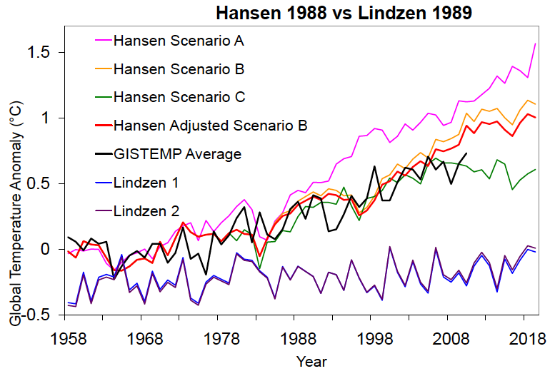
As you can see, Hansen's Scenario B is not far from reality, with a warming trend since 1984 (0.26°C per decade) approximately 30% too high (compared to our average GISTEMP trend of 0.20°C per decade), and the adjusted Scenario B even closer, with a warming trend just 17% higher than observed.

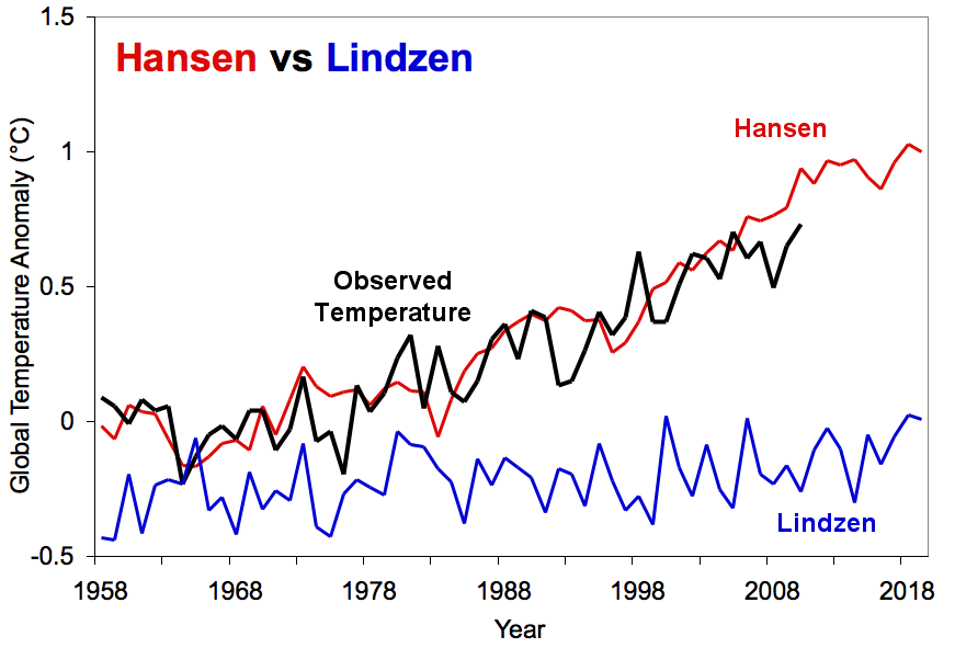
Our reconstructions of Lindzen's projections, on the other hand, increasingly diverge from reality.  His warming trend of approximately 0.01°C to 0.02°C per decade is 90 to 95% too low.  This is further illustrated in the figure below, which isolates the adjusted Scenario B, our second Lindzen reconstruction, and the GISTEMP average (we have also added this figure to the high resolution climate graphics resource page).

Hansen vs. Lindzen projections

Additionally, Dr. Hansen's 1988 climate model was a bit more sensitive to greenhouse gas changes than the models used by climate scientists today, with a sensitivity of 4.2°C for a doubling of CO2.  We can further adjust his Scenario B to reflect the IPCC climate sensitivity of 3°C to determine what today's climate model projections would have looked like in 1988.

Hansen 3°C Sensitivity

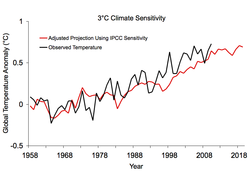
As you can see, the projection matches up very well with the observed temperature increase.  This supports the IPCC most likely climate sensitivity value of 3°C for doubled CO2.

This analysis demonstrates that Hansen has a record of highly accurate climate projections over the past two decades, while Lindzen has a record of inaccuracy.  Indeed, Lindzen continues to argue for low climate sensitivity to this day (not quite as low as 0.3°C, but he continues to argue it's below 1°C for doubled CO2 [i.e. Lindzen and Choi 2009]).

Given all the heat "skeptics" have directed towards Hansen for his projections' slight overestimate of the subsequent warming, one can only wonder what they must think about the massive underestimate of this warming based on Lindzen's 1989 comments.

0 0

Printable Version  |  Link to this page

Comments

Prev  1  2  3  Next

Comments 51 to 100 out of 110:

  1. Regarding the rather bizarre quote posted @50. It so perfectly demonstrates the inanity and fallacy of Lindzen's opinion on this serious issue :) Ironically he is falsely accusing others of the very things that he is guilty of. Lindzen managed to squeeze in at least four misp-representations of the facts and the science in that quote. Whenever he made that quote, he had clearly long since abandoned (and turned his back on) serious science...
    0 0
  2. ...and here we have another denialist trick courtesy of RW1-namely the "appeal to authority". However, given Lindzen's total lack of credibility, appeals to *him* as an authority are liable to receive nothing but gales of laughter from those who treat science more seriously than those in denial. Also, RW1, according to GISSTemp-which actually incorporates polar temperature-temperatures for January to March have averaged around +0.5 degrees above the 1951-1990 mean temperature. This, in *spite* of record cold winters along the Atlantic Coasts, & in spite of an ongoing La Nina. As we've now come out of the La Nina, & are now approaching the NH Summer, I think its fair to say that average temperatures for 2011 will almost certainly be equal to-if not greater than-the average temperature for 2010.
    0 0
  3. Moderator Response @35 Yes there was a robust discussion but there was no misubnderstanding on my part. Your arguement basically is that Scenario C is irrelevant because it does not follow actual emmissions. Therefore, it is a coincidence that real-world temperatures follow it. It is possible that the accuracy of Scenario C is a coincidence. However, if real world temperatures continue to follow it then we will need to re-evaluate our current theories/hypotheses on climate forcing. Scenario B would then become irrelevant. Hansen (2006) suggests that we should be able to differentiate between Scenarios B and C by 2015.
    0 0
    Response:

    [DB] You are basing your misinterpretations on a graphReal life follows physics.  Hansen based his modeled projections for the various scenarios (A, B and C) on a climate sensitivity factor that was too high - for each of the scenarios.

    Adjustment of the sensitivity to what our current understanding shows it to be yields a much tighter fit to the Scenario B track for actual temperatures than it does for Scenario C.  And for down the road, actual emissions diverge widely from the assumptions for Scenario C, so temperatures in the real world will track emissions because of physics, diverging even more widely from those in Scenario C.

    You were told all of this before in the thread referenced in comment #35.  Why you refuse to understand any of it is beyond me.

  4. Actually, RW1's quotation of Lindzen at #50 provides another prediction... that warming will be limited to "a few tenths of a degree". Frankly, this is already false... unless we ignore the thermometer and proxy temperature records and consider only Lindzen's own, much shorter, satellite records. However, even that won't be true in ten to twenty years for the 'future generations' Lindzen speaks of.
    0 0
  5. CBDunkerson @54, " Lindzen at #50 provides another prediction... that warming will be limited to "a few tenths of a degree"." Indeed, that prediction has already been proven incorrect. Moreover, even if one looks at the satellite era (1979 onwards) , there has already been about 0.5 C warming in the lower troposphere during that period (1979-present warming trend +0.163 C/decade in the RSS data). Daniel Bailey @53, "Why you refuse to understand any of it is beyond me." Not that this is news to you, but the reason is very clear to everyone but the person being referred to, and that reason is denial.
    0 0
  6. angusmac @51 Hansen (2006) suggests that we should be able to differentiate between Scenarios B and C by 2015. This statement only refers to the simulations reported in Hansen 2006 which were for the period 2000-2100, it is wrong to conflate Hansen's scenario C from 1988 with his AS from 2006
    0 0
  7. DB (RE: 50), "RW, it is simply unacceptable here to post a quotation without providing both context for the quote and a linked source for the quote. That part of Skeptical Science ain't a-changin', despite the clamor of "skeptics"." The quote is from a recent piece of his entitled "A Case Against Precipitous Climate Action" You can google it if you want to read the whole thing. The quote aside, there is very little going on here with temperature record. The 0.3 C or so upward trend over the last 30 years could easily happen by dumb luck alone. I certainly don't dispute the upward trend or that man's CO2 may have contributed to it at some level, but it isn't very much. Even if we assumed man's CO2 caused 100% of the 32 year trend of 0.3 C, that amounts to only about 1 C of warming over a hundred years.
    0 0
    Response:

    [dana1981] Sure, the warming could be natural variation, if you completely ignore all physics and climate science.  Just like if I start a forest fire, it could have been started by a lightning strike!  Aren't hypotheticals fun?

    For your 1°C warming over 100 years claim, I refer you to Monckton Myth #3: Linear Warming.

  8. Re #57, "Even if we assumed man's CO2 caused 100% of the 32 year trend of 0.3 C, that amounts to only about 1 C of warming over a hundred years." The warming is closer to +0.5 C in 32 years (as per RSS trend of 0.163 C/decade). So 0.163 C/decade translates into another 1.6 C of warming over the next 100 years should the current 32-yr trend continue. Regardless, the observed warming of almost 0.9 C since 1880, and most of that is in response to "only" a 40% increase in CO2 levels. There is just so much wrong with the numbers and logic in the above quote from #57 that it beggars belief.....it also goes to show, you can take people to the science, the data, but you cannot necessarily penetrate ideological barriers.
    0 0
  9. dana1981 (RE: 57), "Sure, the warming could be natural variation, if you completely ignore all physics and climate science. Just like if I start a forest fire, it could have been started by a lightning strike! Aren't hypotheticals fun?" The point is unless the amount of warming is outside the range of natural variability over a given period of time, there is no way to accurately quantify how much of it is due to man. Also, the only genuine first principle derived physics are that of the radiative forcing of CO2 (3.7 W/m^2 per doubling), the measured response of system to incident energy at the surface (about 1.6), and the constraints COE puts on the system.
    0 0
  10. Well I disagree with "no way to quantify", but for outside natural cycles, the calculation has been done and a convenient graphic is here Oh, and first principle physics, how about the quantum basis for radiative adsorption by GHGs?
    0 0
  11. RW1#59: "unless the amount of warming is outside the range of natural variability" That works both ways. Please tell us exactly the range of natural variability and how you obtain that figure. Responses belong on the Natural cycles thread.
    0 0
    Moderator Response: Indeed, responses here will be promptly deleted without warning.
  12. muoncounter (RE: 61) "That works both ways. Please tell us exactly the range of natural variability and how you obtain that figure." Answered here
    0 0
  13. Moderator@53, "Real life follows physics". OK, for the sake of discussion let us assume that your physics is correct. I compare your adjusted Scenario B with Hansen's original scenarios in the figure below and the following points are evident:
    • Your adjusted Scenario B reduces the projected temperature anomaly for 2019 from 1.10°C to 0.69°C. Wow! This is very close to the Scenario C value of 0.61°C.
    • Actual temperatures follow Scenario C much better for the whole period from 1958 to 2010 than your adjusted Scenario B. Your adjusted Scenario B only catches up with Scenario C in 2010. Thereafter it is slightly higher than Scenario C but follows a similar trajectory.
    It would appear to be a case of Scenario C - "wrong" physics: right answer. Your adjusted Scenario B - "right" physics: not so good answer. Incidentally, Hansen stated in 1988 Senate Committee hearing that Scenario A is "business as usual". It would appear from your adjusted Scenario B that this was a "massive" overestimate.
    0 0
    Moderator Response: [mc] Please restrict image width to 500.
  14. Angusmac - close. Scenario C is "different reality", not wrong physics. Scenario B is closest to actual reality and yes, in Hansen's case physics was out. His incredibly primitive model had a sensitivity of 4.2. Better physics in current models estimate sensitivity at 3, and lo, that is what fits with the temperature record. "Adjust" the Hansen prediction to a sensitivity of 3 and that is what you get.
    0 0
  15. angusmac - I'm failing to see your point. If Adjusted Scenaio B is "not so good answer" (looks pretty darn good to me), how would you describe Lindzen's projection?
    0 0
  16. Dana@65, I describe Lindzen's as the worst of all the scenarios presented by you; even the massive overestimate that is Hansen’s Scenario A performs better. Scaddenp@64, my Figure@63 does show Dana's adjusted Scenario B with a sensitivity at 3. However, Scenario C with a sensitivity of 4.2 still gives a better fit with actual temperatures. I agree that the models use comparatively simple physics but this is also why they are extremely useful. There would appear to be something missing in the post-2000 behaviour of Scenario B that is (coincidentally?) captured very well in the excellent empirical performance of Scenario C.
    0 0
    Moderator Response: [DB] And you base this on what model of EyecrometerTM...?
  17. angusmac - I still don't see your point. Yes, scenario C coincidentally fits observed temperatures pretty well. We know it's coincidental because that scenario in no way matches reality. The forcing is lower and the sensitivity is higher. Those two opposite inaccuracies just happen to cancel eachother out. If we bump our adjusted Scenario B up to a sensitivity of 3.4°C, it would match observations better. But I decided it would make more sense to use the IPCC most likely value (3°C). So it seems like if we boil it down, you're arguing that real-world climate sensitivity is on the high side.
    0 0
  18. A model is something which take a inputs "scenario" and get the outputs. You can model say a cannonball, and construct scenarios for elevations of 10,30, and 45 degrees. However, if you actually experiment with an elevation of 30 degrees, why would you be interested in comparison with the 10 and 45 predictions? Comparing with Scenario C is like noting that your 10 degree elevation prediction matched it better because your model overestimated the powder. Simple is useful for education, not real world. By that logic you should love Wally Broecker's pretty spot on prediction of 2010 temperature that he made in the 1970's. However the model used, while actually an amazing thing, makes Hansen's model look seriously sophisticated. A wet sphere (no ocean) dry part on 2/3 of upper hemisphere from memory. Wally overestimated the CO2 (thought we would be at 400) while the model only had a sensitivity of 2.3 from memory. (I'm away from papers). You want real airplanes to be designed from a high school flight model, because it's simple? No. Hansen did what he could within the limitations of the day. You want as much real world physics in there as possible for a good prediction.
    0 0
  19. Moderator@66, your Eyecrometer sounds like a very useful device. Can I buy one on Amazon?

    You already have the post-2000 figures. Scenarios B and C both show a warming trend of 0.26 °C/dec for the 1958-2000 period, however, they diverge post-2000. I show the trends for 2000-2011 here and I summarise them below:

    • Scenario B = 0.38 °C/decade
    • Scenario C = 0.12 °C/decade
    • Real-world (GISS LOTI) = 0.15 °C/decade

    There is a definite dogleg in real world temperatures post-2000.

    I request that you publish the figures for the adjusted Scenario B so that I can incorporate them in my models.

    0 0
    Response:

    [DB] "There is a definite dogleg in real world temperatures post-2000."

    The warmest decade in the instrumental record is a "dogleg"?  Where's the dogleg:

    Ten

    [Source]


    Well, it's not evident in any of the temperature records.  How about since 1975 (removing the cyclical noise & filtering out volcanic effects):

    1975

    [Source]

    No dogleg there.  How about the warming rate estimated from each starting year (2 sigma error):

    CRU

    [Source]

    THe warming since 2000 is significant.  Still no dogleg.

    Your focus on statistically insignificant timescales is misplaced.  While a world-class times-series analyst (like Tamino) can sometimes narrow down a window of significance to decadal scales, typically in climate science 30 years or more of data is used.

  20. Dana@67, I am not arguing for higher sensitivity.

    I just find it ironic that SkS can praise the accuracy of Hansen's 1988 projections without mentioning the dramatic drop in temperature projections. Here is a timeline derived from SkS blogs for Hansen's 2019 temperature anomaly:

    • Hansen (1988): Scenario A is "business as usual." Anomaly = 1.57°C.
    • Hansen (2006): Scenario B is ''most plausible.'' Anomaly = 1.10°C.
    • Dana (2011) in this blog: Adjusted Scenario B "matches up very well with the observed temperature increase." Dana is silent on the anomaly but the blog's chart indicates that Anomaly = 0.69°C.

    In summary, SkS have presented many blogs praising the accuracy of Hansen (1988) but have neglected to mention that the Hansen's original projection for the 2019 temperature anomaly has plummeted from 1.57°C in 1988 to 0.69°C in Dana (2011). Why is this not mentioned?

    Dana, I find it difficult to believe that these plummeting temperatures have not escaped your attention. Do you have a problem with declaring that your adjusted Scenario B is only slightly above Hansen's zero-emissions Scenario C?

    0 0
  21. Scaddenp @68, you misrepresent me by stating that, "You [I] want real airplanes to be designed from a high school flight model, because it's simple?"

    Real engineers and scientists use simple models every day to check the validity of their more complex models. They usually use simple physics to check if small changes in their assumptions lead to large changes in outcomes.

    Dana in this blog used a simple spreadsheet to adjust Hansen's Scenario B without the need to re-run the whole computer model.

    0 0
  22. Angusmac, I have no problem acknowledging Hansen's 1988 prediction were out because the primitive model has a sensitivity that was too high. However, given the uncertainties in determining climate sensitivity, I think it was a pretty good effort for its time. Both history and better model show a convergence on sensitivity of 3.
    0 0
  23. angusmac, you're misrepresenting the facts. Maybe Hansen described Scenario A as the result if we continued with "business as usual", but the fact is that the radiative forcing has been nowhere near that in Scenario A. Hansen is not in the business of predicting how GHG emissions will change, he's in the business of projecting for a given GHG change, how much temps will change. That's what the adjusted Scenario B represents. Your claimed "dramatic drop in temperature projections" is purely imagined. That's why it's not mentioned.
    0 0
  24. Moderator@69, a temperature trend of 0.26°C/decade pre-2000 and 0.15°C/decade post-2000 (GISS LOTI) is a dogleg. Your last chart also shows the dogleg with figures of 0.02°C/year for start dates of 1990 and earlier and 0.01°C/year for start dates of 2000 and later. A renowned climate scientist (Hansen, 2006) stated that we should be able to distinguish between Scenarios B and C within a decade (see below): Within a decade is by 2015. However, if you consider this period to be statistically insignificant then I suggest that you argue with Hansen. Incidentally the no-increase-in-emissions Scenario C gives an even hotter decade than real-world "hottest decade on record" (GISS LOTI).
    0 0
    Response:

    [DB] This has been clarified for you multiple times on several threads.  Your persistence and determination in maintaining your narrative in spite of all evidence and physics to the contrary is admirable, but misplaced. 

    I don't mind continually reinventing the wheel to enable learning, but I draw the line at reinventing the flat tire.

  25. Dana@73, "Your claimed dramatic drop in temperature projections is purely imagined." I disagree. It is not imagined it is fact. Let me explain as follows. In this blog you compare Hansen (1988) with Lindzen (1989). What Hansen and Lindzen said then is particularly relevant. Hansen (1988) in his congressional testimony described Scenario A as “business as usual” (see below). In effect, Hansen told Congress in 1988 that the temperature anomaly for 2019 would be circa 1.57°C. This is a fact. Later (2006), Hansen was economical with the truth when he re-worded his 1988 congressional testimony to be Scenario A, "was described as on the high side of reality." Dana the facts are that the 2019 temperature anomaly has been amended downwards from 1.57°C in Hansen (1988) to 0.69°C in this blog. Furthermore, your adjusted Scenario B has reduced the Hansen's Scenario B anomaly from 1.10°C to 0.69°C but you neglected to mention this fact. Surely this temperature drop can be described as dramatic? Finally, I would be pleased if I could have a response to my question in angusmac@70. Do you have a problem with declaring that your adjusted Scenario B is only slightly above Hansen's zero-emissions Scenario C? 0.69°C for your adjusted Scenario B and 0.61°C for Hansen's original Scenario C seem pretty close to me.
    0 0
  26. Dana, Believe it or not, the above obfuscation has given me an idea. I'll try and post about it this weekend. Basically what it boils down to is that these data suggest that a sensitivity of +3 K may be somewhat too low.
    0 0
  27. angusmac - as I've said, climate scientists aren't in the business of predicting how emissions will change. That depends on policymakers, not physics. Perhaps if emissions had continued to accelerate at the rate they were in 1988, Scenario A would have become reality. Regardless, nothing was "amended downward". A different scenario became reality. Yes, coincidentally when adjusting Scenario B to reflect 3°C sensitivity, current temp projections come close to Scenario C with 4.2°C sensitivity. I think it's kind of silly to obsess over coincidences though.
    0 0
  28. Albatross - I kind of tried to make that point, that with this data, the most likely sensitivity is actually closer to 3.4°C.
    0 0
  29. angusmac seems to be woefully lost in the difference between a scenario -- a set of preconditions on which to base a projection -- and the projection resulting from that scenario. He wants to argue that Scenario X is the right one because the end result matches observations, without regard to the fact that the conditions underlying Scenario X never came to pass. He then further obfuscates things by using the 10-year-old description of a scenario (such as "business as usual" for Scenario A) as an argument that it should apply today (because we currently describe what we've done since 1998 as "business as usual"). It's all really a very clever misunderstanding. angusmac, here are some basic facts that point out the major fallacies in your comments to date: 1) Scenarios A, B, and C represent emissions growth patterns, not temperature predictions. 2) Hansen's own description of those scenarios at the time was this:
    Scenario A assumes continued exponential trace gas growth, scenario B assumes a reduced linear linear growth of trace gases, and scenario C assumes a rapid curtailment of trace gas emissions...
    Note the use of the word "continued," which is sort of like "business as usual," but I hope that you can appreciation the difference. 3) Actual emissions growth since 1998 has been linear (i.e. scenario B) even though at that time the pattern had been exponential, and would have matched scenario A. This makes scenario B the best match to actual events for the emissions on which each projection is based 4) So whatever projection went with scenario B (which more closely matches actual emissions) is the one we should consider. 5) Since that projection accompanied a pattern of emissions which never came to pass (i.e. scenario B is closest to, but not equal to, actual emissions since 1998) it is fair to adjust the projection in a minor fashion to more closely match what it might have said, had scenario B matched actual emissions. Which of these rather simple points still eludes you?
    0 0
  30. I would point out that since angusmac has argued that Scenario C most closely matches observed temperatures, and therefore by his logic is the correct one to consider... ...he has in turn proven that actual CO2 emissions since 1998 have represented a rapid curtailment of trace gas emissions (Hansen's 1998 words). angusmac has successfully proven that we've already abandoned fossil fuels, and so there is no longer any danger of climate change. Let me be the first to congratulate everyone on a job well done. Humanity, and civilization, are saved by a simple and convenient re-interpretation of history. I wish I'd thought of that.
    0 0
  31. Sphaerica@80, in which you state that, "Humanity, and civilization, are saved by a simple and convenient re-interpretation of history." There is no re-interpretation just a bald statement of historical measurements which show that the GISS LOTI real-world temperatures match Scenario C better than the other scenarios. If those pesky people at GISS choose to publish figures that are too low to comply with your preferred warming scenarios then it is not my fault. @79"Scenarios A, B, and C represent emissions growth patterns, not temperature predictions." I disagree. Hansen, in his 1988 congressional testimony, concentrated almost exclusively on discussing higher temperatures and the dire consequences of his (global) warming predictions. Similarly, Hansen (1988), quoted by you, expends most effort on temperature predictions and consequences thereof. He only expends one-third on emissions. DB @74, "This has been clarified multiple times on several threads." Not so. There have been many statements in SkS that Scenario C does not follow real-world emissions and consequently is irrelevant. There have been no clarifications; just repetition of the mantra that Scenario C is either irrelevant or a coincidence. I ask a simple question, how long does it take for a scenario that is nominally a coincidence to become reality? See below. Albatross@76 and Sphaerica@79, the Cambridge Dictionary defines to obfuscate as, "to make something less clear or harder to understand, especially intentionally." What could be clearer to anyone than the real-world emissions being significantly above Scenario C but real-world temperatures (GISS LOTI) following Scenario C? There is no obfuscation just a bald statement of facts. Yet, SkS repeatedly state that this is coincidence. Question: I repeat, how long does it take for a coincidence to become reality? Answer: I agree with the Hansen (2006) estimate that 2015 would be long enough to differentiate between the scenarios. This represents a period of 27 years from 1988 to 2015 but DB@74 seems to think that this is reinventing the flat tyre [I don't get the allusion]. If the real world is still following Scenario C in 2015 then there would need to be a rethink of climate sensitivity and/or forcings. Is this why SkS is so vehement in stating that Scenario C is a coincidence? Sphaerica@79, if I were to use your Scenario X with the following figures: Temperature Anomaly = 0.015175 x Year - 29.903 I would have an excellent model for the temperature anomaly between 2000 and 2011. Furthermore, if were to use this model to predict the anomaly for 2019 to be 0.74°C, and this prediction turned out to be correct, then you would have to agree that I had quite a skilful temperature model. Yet, there are no emissions used in this model. This would be a case of a dumb (empirical) model giving good results. If real-world physics gives poor results then I suggest that we need to re-examine the physics to give better results. Dana has started this process. The 3°C sensitivity model appears to give better results than Hansen's original Scenario B. It predicts 0.69°C for 2019 compared with 0.61°C in Scenario C. However, do be aware that this is not a "minor" change. This is a massive drop from the 1.10°C in original Hansen's Scenario B.
    0 0
  32. angusmac -
    "how long does it take for a coincidence to become reality?"
    This is a bizarre question. How long does it take a hypothetical scenario which is not reality to become reality? An infinite amount of time. Unless you invent a time machine, go back to the late 20th century, convince them to phase-out GHG emissions, and then alter the global climate such that it has a short-term sensitivity of 4.2°C. If you can do that, Scenario C will become reality. Look, there are an infinite number of possible scenarios you could model. A large number would match observed temp changes reasonably well. But only one scenario matches reality, and it's not Hansen's C. That's just one of the many possible scenarios that so far match observed temps reasonably well. But we know it's wrong because we've measured the actual radiative forcing to a high degree of accuracy. There is simply no way Scen C matches reality. It just doesn't (unless you invent that time machine and a way to change the planet's sensitivity). There's a phrase "skeptics" like to use but don't seem to understand that it applies to their arguments too: correlation does not equal causation.
    0 0
  33. I should also note in comment #70 you said "I am not arguing for higher sensitivity." Then in comment #81 you asked "how long does it take for a coincidence to become reality?" If Scenario C "becomes reality", then climate sensitivity is 4.2°C for 2xCO2. So contrary to your previous claim, you are indeed arguing for high climate sensitivity.
    0 0
  34. Hi Dana, Thanks for #78, that is what I was driving at. I'm not sure how people are trying to take away solace from these findings. A climate sensitivity of +3 K does not bode well for society, especially given that we will very likely easily double CO2. I see what is going on here, every effort must be made to obfuscate (and yes I do understand what it means angusmac) and detract form Lindzen's "prediction". Really, who do me trust, Lindzen who is an order of magnitude out or the science which has converged on +3 K for climate sensitivity, and a value which is in fact seems to produce temperatures that are a tad on the low side, with +3.5 or so providing the "best" fit using the observed radiative forcing, at least for these data. Now, what might help address some of the confusion (although I'm still not convinced the confusion in some quarters is innocent in nature) is a graphic (much easier to interpret than numbers) showing the observed radiative forcing since 1958 to present, together with the radiative forcing for the various scenarios. That will hopefully make is abundantly clear to certain "skeptics" that the relatively good agreement between Scen C is coincidence, or perhaps more accurately, the more-or-less correct answer for the wrong reasons.
    0 0
  35. Global surface air temperature (SAT) anomalies in the GISTEMP data for 2010 were 0.63 above the 51-80 baseline. I expect the global SAT anomaly to be between 0.80 and 0.85 C in 2020, compared to about +0.70 using a sensitivity of +3 K and best estimate of emissions between now and then. And now the elephant in the room-- using Lindzen's reasoning, we should expect a global SAT anomaly relative to the 51-80 baseline of just under 0 C in 2020, in other words still in negative territory! That is not surprising, b/c values based on his reasoning have been diverging from reality since the early eighties. Interestingly, that occurred before he made his comments in 1989 that are cited above.
    0 0
  36. Alby #84 - Gavin made a figure similar to what you're asking for, though it's a little out of date:
    0 0
  37. Thanks Dana, I think that figure @86 makes things abundantly clear. Maybe an updated version would be a useful addition to the main post?
    0 0
  38. Dana@83, "contrary to your [my] previous claim, you [I] are indeed arguing for high climate sensitivity." This statement is incorrect and you are aware of it. I state that Scenario C predicts real-world temperatures very well. This scenario has no increase in forcing after 2000 and therefore it has zero temperature rise for 2000-2019 irrespective of the sensitivity value. ( -Snip- )
    0 0
    Response:

    [DB] Accusation of mendacity snipped.  You are free to disagree, angusmac.  But do not accuse others of lying when it is readily apparent that you either:

    1. Just don't understand the subject matter
    2. Are intentionally only looking at information which agrees with your understandings and ignoring everything else.

    In any event, many have wasted their time trying to help you gain a better understanding of the matter.  I suggest, if the answers here are not to your liking, a different venue might be in the offing for you to gain the clarity you seek.

  39. angusmac - nope sorry, Scenario C would not match up well with the temperature rise if not for the 4.2°C sensitivity. Your whole point is that Scenario C "looks good". It wouldn't look good without high sensitivity. You can't just ignore the aspects of the scenario and model that you don't like. You don't get to have your cake and eat it too. Clearly you don't want to argue for high climate sensitivity, but that is nevertheless exactly what you're doing. Or more accurately, you're arguing for an alternative reality in which one aspect is high sensitivity.
    0 0
  40. Dana@86, I agree with Albatross. Your diagram makes the forcings absolutely clear. However, let me try to make it clearer by adding temperatures. Two observations are evident: • Scenario B temperature predictions are in good agreement with real-world forcings but they fail miserably when compared with real-world temperatures. • Real-world temperatures do not follow real-world forcings. However, they are in good agreement with the dogleg forcings and temperatures of Scenario C. Dana, I totally agree that "correlation does not equal causation". However, Hansen (2000) offers an alternative scenario that would change the "bizarre" coincidence of Scenario C into reality and also providing causation. Hansen suggests that the effects of anthropogenic aerosols could balance CO2 forcings. However, he does note that this is a wild card and that current trends are uncertain. I show the forcings from Hansen's alternative scenario below. Figure 1: A scenario for additional climate forcings between 2000 and 2050. Reduction of black carbon moves the aerosol forcing to lower values (Hansen et al, 2000) Hansen's 1988 scenarios only consider CO2, CH4, N2O, CFC11 and CFC12. However, it is evident from Figure 1 that the largest anthropogenic climate forcing (due to CO2) could be reduced by negative forcings from aerosols. Perhaps this is the reason why Scenario C gives good results? If we plugged the negative forcings from aerosols into Scenario B it would result in similar forcings to Scenario C. We would then change the coincidence of Scenario C into a reality of new Scenario B. This new scenario would be able to simulate the post-2000 temperature flattening that is so well modelled by Scenario C. Tropospheric aerosols look to be the likeliest candidate for a reduction in the CO2 forcing in Scenario B. China and India have seen huge growth in the last 10 years, most of which is founded on industries that produce large quantities of aerosols. These countries also represent half of the world's population. Therefore, it is not difficult imagine that their aerosol emissions would dwarf Gavin Schmidt's 1940s aerosol blip. Consequently, it is likely that they produce enough negative forcing to cancel out the CO2 forcing in Scenario B thus allowing it to conform to real-world temperatures.
    0 0
  41. angusmac - I really don't understand what you are going on about. Hansen's 1988 model had a climate sensitivity that was (in hindsight) far too high - 4.2°C, rather than ~3°C/doubling of CO2. It was run on three different emissions scenarios, which are not predictions of economic and political action, but rather guesses, to see how the model would evolve in temperature. Now, many years later, the emissions that actually occurred are closest to Scenario B. Taking Hansen's (rather simple, by today's standards) 1988 model and re-running it with Scenario B emissions and a sensitivity of 3°C/doubling of CO2 matches the actual progression of temperatures surprisingly well. And if you use actual emissions (slightly different than Scenario B), Hansen's model has a best match at a climate sensitivity of 3.4°C/doubling. That's pretty amazing for an early model - Hansen is to be congratulated! Scenario C? That didn't happen, and is hence irrelevant to current conditions. The only way you see the match to Scenario C you are going on about is if you keep the 1988 sensitivity of 4.2°C/doubling, which has been shown not to be a reasonable estimate. So - you're arguing about an emissions scenario that did not occur, and how that matches to a climate model run with a sensitivity that later proved incorrect. Why are you wasting your time, and everyone elses, with this?
    0 0
  42. angusmac - aerosols are taken into account in Schmidt's and my analyses. You're eyeballing and speculating. I ran the actual numbers.
    0 0
  43. KR - angusmac is trying to find a way in which Scenario C, which doesn't reflect reality, could reflect reality. He seems completely unwilling to accept the fact that it is not an accurate scenario. I think continuing to try and explain this is a waste of time.
    0 0
  44. Dana@92, I would be pleased if you would supply your numbers for review.
    0 0
  45. KR@91, I have run some statistical checks (Dana not the eyecrometer) and I confirm that Dana's 3°C scenario gives good results. Almost as good as Scenario C. Therefore, I might use it for future temperature comparisons to save all the hassle about Scenario C not being "real". Dana@93. No I wasn't trying to, ""find a way in which Scenario C, which doesn't reflect reality, could reflect reality."" Scenario C already gives the right temperatures. I was actually trying to suggest an alternative method of getting Scenario B to reflect reality. I still haven't received your figures to show aerosols are taken in to account in Scenario B. Nevertheless, I have downloaded your spreadsheet (which doesn't show aerosols) from SkS Graphics Resource (this is a good resource and excellent FOI) and as I said to KR above your 3°C scenario gives good results. However, I make the following comments:
    • The sensitivity is actually 2.7°C because you have left the 0.9 x 3.0 factor in your calculations.
    • You splice your 2.7°C sensitivity to the 4.2°C Scenario B. This is illogical but I assume that you did this because Gavin Schmidt (2007) at RC states that you should start analyses at 1984 to avoid a "cold start". However, I see no reference to the "cold start" in any of Hansen's papers. To the contrary, Hansen (1988) explains that 1959 was chosen as his best estimate of climate equilibrium. Nevertheless, using 1959 as a start date increases the temperature projections by approximately 2% and gives you a better fit with real-world temperatures.
    0 0
    Response:

    [dana1981] You're mistaken.  The 0.9 is to account for the fact that the observed radiative forcing (which includes aerosols) is 10% lower than Scenario B.

  46. Dana, to summarise our discussuion, I enclose the timeline and narrative showing the reduction in the estimate for the 2019 temperature anomaly from Hansen's initial estimate of 1.57°C in 1988 to your estimate of 0.69°C in 2011. Links: Hansen (1988a), Hansen (1988b), Hansen (2005), Hansen (2006), Schmidt (2007) & Dana (2011)
    0 0
  47. Angumusac Pretty elaborate table. You could summarize it in two sentences though. 1. Hansen's early model had too high a sensitivity. 2. Scenario B ended up with the forcing that best matched reality out of the three. Why not just say that?
    0 0
    Response:

    [dana1981] Because he's trying to exaggerate how far off Hansen was by using this "business as usual" quote, even though it's been explained to him several times that Hansen is not in the business of predicting future CO2 changes.

  48. I'd like to suggest to any casual readers that they look at angusmac's posts, and those in response, and note how he quite simply refuses to see the point of the entire argument. He is so intent on proving a point that he desperately wants to be true that he is ignoring the simple and obvious... even after it has been explained to him over and over again. This is an important behavior to watch for on these threads, the habit of some to make their case by mere repetition, often through the inclusion of as many numbers and graphs and equations as possible, while simply and blatantly ignoring even the most basic and irrefutable arguments that knock the supports right out from under their case. Merely repeating a flawed argument over and over, with more and more intricate (if invalid) numbers, does not make it any more true, or convincing, and forcing others to repeat the same salient point over and over does not make that point any less true. Be wary.
    0 0
  49. Actually, is angusmac trying to imply that since he thinks scenario C is a good fit for actual temperature then the forcings are actually close to scenario C???
    0 0
  50. I think the idea that actual forcings may match scenario C closer than scenario B is intriguing. A lot depends on the aerosol forcing, which is the only reasonable candidate for causing a flattening of forcing since 2000. As far as my google skills and level of patience can tell,there is no direct measurement of aerosol forcings. I have found a paper from 2004 discussing the need for such measurement. http://glory.gsfc.nasa.gov/publications/2004_JQSRT_88_149.pdf So if there is no direct measurement, that must mean that aerosol forcings used in models such as GISS E are indirect estimates based on calculations such as looking at economic activity etc? A few years ago I made an amateur attempt at trying to indirectly calculate aerosol forcings using Co2 emission data. Assuming that aerosol emissions and Co2 emessions have grown at the same rate and guessing some parameters to match total changes in aerosol forcings over the last century, and the claim I have read that most aerosols only last in the atmosphere for about 3 years, I was able to generate a forcing profile that peaks around 2002 and actually decreases for a few years. This is due to the explosive growth in activity in China in the last decade, and the fact that due to the 3 year lifespan of aerosols, aerosols react much faster to changes in economic activity than Co2 does. This crude analysis of course did not take into account the effects of clean air legislation, but I would expect that as the recent growth in emissions is largely in China that this would not be an issue? If the China effect really is the cause of a dog-leg in forcings, and forcings really do follow scenario C, then this will not last. Due to the short life time of aerosols, Co2 accumulation from the China boom will steadily overcome the short term aerosol effect and the forcing will steadily rise to meet and maybe overtake scenaerio B in the next decade or so.
    0 0

Prev  1  2  3  Next

You need to be logged in to post a comment. Login via the left margin or if you're new, register here.


The Consensus Project Website

THE ESCALATOR

(free to republish)


© Copyright 2024 John Cook
Home | Translations | About Us | Privacy | Contact Us