Climate Science Glossary

Term Lookup

Enter a term in the search box to find its definition.

Settings

Use the controls in the far right panel to increase or decrease the number of terms automatically displayed (or to completely turn that feature off).

Term Lookup

Settings


All IPCC definitions taken from Climate Change 2007: The Physical Science Basis. Working Group I Contribution to the Fourth Assessment Report of the Intergovernmental Panel on Climate Change, Annex I, Glossary, pp. 941-954. Cambridge University Press.

Home Arguments Software Resources Comments The Consensus Project Translations About Support

Bluesky Facebook LinkedIn Mastodon MeWe

Twitter YouTube RSS Posts RSS Comments Email Subscribe


Climate's changed before
It's the sun
It's not bad
There is no consensus
It's cooling
Models are unreliable
Temp record is unreliable
Animals and plants can adapt
It hasn't warmed since 1998
Antarctica is gaining ice
View All Arguments...


Username
Password
New? Register here
Forgot your password?

Latest Posts

Archives

CO2 emissions change our atmosphere for centuries

What the science says...

Individual carbon dioxide molecules have a short life time of around 5 years in the atmosphere. However, when they leave the atmosphere, they're simply swapping places with carbon dioxide in the ocean. The final amount of extra CO2 that remains in the atmosphere stays there on a time scale of centuries.

Climate Myth...

CO2 has a short residence time

"[T]he overwhelming majority of peer-reviewed studies  [find] that CO2 in the atmosphere remained there a short time." (Lawrence Solomon)

The claim goes like this:

(A) Predictions for the Global Warming Potential (GWP) by the IPCC express the warming effect CO2 has over several time scales; 20, 100 and 500 years.
(B) But CO2 has only a 5 year life time in the atmosphere.
(C) Therefore CO2 cannot cause the long term warming predicted by the IPCC.

This claim is false. (A) is true. (B) is also true. But B is irrelevant and misleading so it does not follow that C is therefore true.

The claim hinges on what life time means. To understand this, we have to first understand what a box model is: In an environmental context, systems are often described by simplified box models. A simple example (from school days) of the water cycle would have just 3 boxes: clouds, rivers, and the ocean.

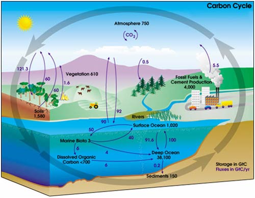
A representation of the carbon cycle (ignore the numbers for now) would look like this one from NASA.

In the IPCC 4th Assessment Report glossary, "lifetime" has several related meanings. The most relevant one is:

“Turnover time (T) (also called global atmospheric lifetime) is the ratio of the mass M of a reservoir (e.g., a gaseous compound in the atmosphere) and the total rate of removal S from the reservoir: T = M / S. For each removal process, separate turnover times can be defined. In soil carbon biology, this is referred to as Mean Residence Time.”

In other words, life time is the average time an individual particle spends in a given box. It is calculated as the size of box (reservoir) divided by the overall rate of flow into (or out of) a box. The IPCC Third Assessment Report 4.1.4 gives more details.

In the carbon cycle diagram above, there are two sets of numbers. The black numbers are the size, in gigatonnes of carbon (GtC), of the box. The purple numbers are the fluxes (or rate of flow) to and from a box in gigatonnes of carbon per year (Gt/y).

A little quick counting shows that about 200 Gt C leaves and enters the atmosphere each year. As a first approximation then, given the reservoir size of 750 Gt, we can work out that the residence time of a given molecule of CO2 is 750 Gt C / 200 Gt C y-1 = about 3-4 years. (However, careful counting up of the sources (supply) and sinks (removal) shows that there is a net imbalance; carbon in the atmosphere is increasing by about 3.3 Gt per year).

It is true that an individual molecule of CO2 has a short residence time in the atmosphere. However, in most cases when a molecule of CO2 leaves the atmosphere it is simply swapping places with one in the ocean. Thus, the warming potential of CO2 has very little to do with the residence time of individual CO2 molecules in the atmosphere.

What really governs the warming potential is how long the extra CO2 remains in the atmosphere. CO2 is essentially chemically inert in the atmosphere and is only removed by biological uptake and by dissolving into the ocean. Biological uptake (with the exception of fossil fuel formation) is carbon neutral: Every tree that grows will eventually die and decompose, thereby releasing CO2. (Yes, there are maybe some gains to be made from reforestation but they are probably minor compared to fossil fuel releases).

Dissolution of CO2 into the oceans is fast but the problem is that the top of the ocean is “getting full” and the bottleneck is thus the transfer of carbon from surface waters to the deep ocean. This transfer largely occurs by the slow ocean basin circulation and turn over (*3). This turnover takes 500-1000ish years. Therefore a time scale for CO2 warming potential out as far as 500 years is entirely reasonable (See IPCC 4th Assessment Report Section 2.10).

Intermediate rebuttal written by Doug Mackie


Update July 2015:

Here is the relevant lecture-video from Denial101x - Making Sense of Climate Science Denial

Last updated on 5 July 2015 by pattimer. View Archives

Printable Version  |  Offline PDF Version  |  Link to this page

Argument Feedback

Please use this form to let us know about suggested updates to this rebuttal.

Update

Updated 'the skeptic argument' on 02/05/2012 to correct formatting errors

Comments

Prev  1  2  3  4  5  

Comments 101 to 121 out of 121:

  1. Eric (skeptic) @98: 1) You where correct that I was ignoring the uptake of CO2 by the land surface/biosphere, which accounts for approximately half of annual draw down of CO2 from the atmosphere. For the reasons given in 97, it is likely that much of that process depends on a rapid establishment of equilibrium on a time scale of from one year to at most a decade. Most likely, in fact, it involves several rapid processes that, but probably also a few slow processes which account for only a small part of the annual effect. In that way, the land would behave similarly to the water in which one rapid, and three slow processes are involved. In that event, the rapid processes would be governed by annual emissions, but the slow processes would be governed by cumulative excess of CO2 (see 3 below). But I don't know enough about the processes involved to make more than these theoretical points. 2) Archer and Brovkin write:
    "A typical ocean surface mixed layer is 100 m deep, and it will equilibrate with the atmosphere (that is, take up as much CO2 as it will) in about a year. But most of the volume of the ocean is beneath the surface layer, and to get there, fossil fuel CO2 has to wait for the overturning circulation of the ocean, which takes centuries or a millennium. Of the 9 Gton C/year carbon release from fossil fuels and deforestation from the year 2000 to 2006, 5 Gton C/year is taken up naturally, half by the ocean and half into the terrestrial biosphere (Canadell et al. 2007). One might conclude from these numbers that the uptake time for CO2 must be only a few years, but this would be a misconception. The rate of natural CO2 uptake in any given year is not determined by the CO2 emissions in that particular year, but rather by the excess of CO2 in the atmosphere that has accumulated over the past century. The lifetime of the CO2 can be gauged by the amount of time that the CO2 has been waiting, which is longer than just a few years. The models find that CO2 peak will come and fade on a time scale of a few centuries to millennia."
    (My emphasis) Clearly from the emphasised sentence, Archer and Brovkin agree with my claim that:
    "[W]hat the environment does is restore equilibrium between the partial pressure of CO2 in the atmosphere and the partial pressure of CO2 in the upper layer of the ocean. That is a rapid process, ..."
    There remains the second quoted paragraph (ie, the paragraph you quoted) which could be interpreted to agree with you. Such an interpretation would be a misinterpretation, however, for by 'uptake' Archer and Brovkin mean the process whereby equilibrium is established between the deep ocean and the ocean surface/atmosphere. Because of the slow transfer of CO2 from surface to the deep ocean, the rate at which equilibrium is established with the deep ocean is indeed governed by the cumulative excess above equilibrium levels accumulated by the surface of the ocean, and the atmosphere. (Because the surface and atmosphere equilibriate over a very short time span, Archer and Brovkin, they mention only the atmosphere.) In contrast, establishing equilibrium between ocean surface and the atmosphere is governed annual emissions. On your interpretation of Archer and Brovkin, they flat out contradict themselves within two paragraphs by claiming that Now you may require something more than the fact that on your interpretation of Archer and Brovkin that the ocean surface and atmosphere will equilibrate within a year, but that 'uptake' will "come and fade on a time scale of a few centuries to millennia". That fact should be enough to see that my interpretation of Archer and Brovkin is correct. But to drive home the point, we see in an earlier passage that they definitely use 'uptake' to refer to the slow, centennial scale process of equilibrating between ocean surface/atmosphere and the deep ocean rather than the rapid process of equilibrating between ocean surface and atmosphere: "To make matters worse, the rate of CO2 uptake by the oceans is much slower than might be inferred from the large surface area of the oceans. Only a small area of the ocean communicates with the largest “pool” of water, the deep sea. Therefore the equilibration time between the atmosphere and the ocean is several centuries, much longer than one might naively expect by simply looking at a globe, or at a “blue planet” photograph from space." Ironically, your misinterpretation means you have quoted Archer and Brovkin in suport of just the error they were warning against. 3) Because there are two processes, equilibrating with the surface layers, and equilibrating with the entire ocean, they can and do operate at different scales and with different drivers. In particular, because the surface layers equilibrate with the atmosphere within a year or so, it is the change in pCO2 from year that drives that process. But the atmosphere can equilibrate with the surface layers while becoming further and further out of equilibrium with the deep ocean. Consequently it is the later disequilibrium that drives the slow draw down of CO2 after the initial establishment of near equilibrium with the surface layer. Two important points arise from this distinction. First, it is the establishment of equilibrium with the surface layers that governs the annual response, and hence the absorption of ~25% of the annual emissions by the ocean. Second, the rapidity of that process cannot be assumed to determine the rate of the establishment of equilibrium with the whole ocean. 4) You can agree that my interpretation of Archer and Brovkin is correct, without agreeing that they or I have established what we claim. Therefore we ought to look at a plot of the CO2 absorbed as a function of annual emissions, and the CO2 absorbed as a function of Annual CO2 concentration - the pre-industrial average. If am correct, the former will show a better correlation to a constant value; while if you are correct, the later will. Conveniently Hansen and Sato 2004 plot exactly those things. (Actually the plot "Airborne Fraction" but annual absorption is just 100%-Airborne Fraction, so the test is equivalent.) I will comment on the 7 year mean as a means of excluding the large amount of noise. Clearly both plots A and C have a number of small excursions from a constant value, no doubt attributable to fluctuations in global temperature and/or ENSO. Both also have a large excursion in the early 90's, no doubt attributable to the rapid cooling consequent on the major volcano at that time (Pinatubo?). But the plot of the draw down of CO2 against cumulative change in CO2 concentration shows two additional large excursions, one at the start, and one at the end, which are not present in the plot against a constant fraction of annual emissions. Clearly then, the available evidence supports my (and Archer and Brovkin's) understanding over yours. While I doubt the evidence is conclusive, given the noisy nature of the data, none-the-less your position means you are arguing against both the evidence, against straightforward theoretical considerations, and against expert opinion. In that position, I would have very little confidence of the correctness of my position. 5) Finally, you quote the seasonal variation in CO2 concentrations as a disproof of my position. However, it is plain that the seasonal variations have a half cycle significantly less than the typical time to reach equilibrium with the surface. Therefore, while we would expect interactions with the ocean to dampen, we would not expect them to eliminate the cycle. Further, given that about a quarter of the annual emissions are absorbed by land, which violently fluctuates in temperature, moisture, and coverage over the course of the seasons, the land based processes may dampen, be neutral with, or amplify such a cycle. Given this, and given the lack of knowledge regarding the land based processes, and given that you cannot quantify the actual amount of CO2 emitted by decay of biota over Autumn and Winter so that we cannot predict the size of the cycle except by measuring it; we simply do not have enough information to run the argument you are trying to run. That does not mean I have refuted this argument. But it does mean you have not provided a reason to disagree with the balance of evidence which is strongly against your position.
  2. Tom, on point 5, if my argument is void because "seasonal variations have a half cycle significantly less than the typical time to reach equilibrium with the surface", then it seems that it would also void your argument that 50% of fossil fuel contribution is soaked up each year, rather than roughly 2% of the excess over full system equilibrium. It is the reality of full system equilibrium (not just surface ocean0 that allows the consistent soaking up of CO2 year after year. Simply put, the top layer ocean carbon has to go somewhere each year so that the top layer can soak up more the next year. The only possible place is the deep ocean and it must have been consistent the past 100 or more years to reach the level we are now at given all those past releases. We have the needed data to quantify the actual amount of CO2 emitted by the decay of the NH biosphere in autumn. It is in the paper that I referenced. I could not provide a link since I had to purchase the paper, but here's the abstract: http://www.agu.org/journals/ABS/1997/97GB02268.shtml I'd be happy to send the paper if you want me to upload it or send it somewhere. For your point 2, I did take Archer and Brovkin somewhat out of context. But their context is not as simple as you suggest, an equilibrium between the deep ocean and top layer / atmosphere. That is not a slow process as you suggest and they imply. The main reason they get away with that implication is that they are adding warming feedbacks to the analysis without explicitly saying so (although it is obvious from the rest of the paper). The deep ocean and top layer have a sufficiently rapid exchange to sequester roughly 40% of the warming expected in the atmosphere / top layer from AGW. That same turnover sequesters CO2. But that also fills the deep ocean reservoir which is the other (an important) reason for the very long tail described by Archer and the graphs earlier in this thread. My essential point in the carbon sequestration process is that CO2 can drop half way back to preindustrial in 50 years as shown in my spreadsheet and .the charts in this thread. The reason it is able to do that is relatively rapid deep ocean sequestration. Archer does not fundamentally contradict that, but he does posit lots of changes to that rate based mainly on warming (also acidification). I think that point also argues against your point 3. I think your charts A and C in your point 4 don't contradict either of our positions. It can be visualized either way, the 40% of annual emissions that are absorbed or the 1.6% of total anthropogenic carbon that is absorbed. The real question is, what does the carbon system do, does it quickly absorb the annual anthropogenic CO2 into the top layer for a variety of effects including acidification and deep ocean sequestration? Or does it behave more simply as a deep ocean sequestration system albeit with a rapid top layer interface, but the long term rate (1.6%) being determined by the deep ocean turnover? I think the answer is both are true because across the world from the tropics to the arctic, the ocean are doing all of the above all of the time. There are always places with lots of deep ocean sequestration (e.g. the arctic before freezeup) and places with very little (the tropics most of the time). The mix of those conditions is what supports the current atmospheric levels over the long run but the multi-year changes in that mix is what also causes the fluctuations seen in the charts you posted.
  3. Eric (skeptic) - Regarding speed of CO2 uptake, I would strongly suggest you take a look at the IPCC report, Section 7.3, The Carbon Cycle and the Climate System, and in particular 7.3.4.5 Summary of Marine Carbon Cycle Climate Couplings, where this is discussed. Given that the various mechanisms (uncertain as to positive/negative feedbacks) have time ranges from 1 year to 50K years, with high capacity negative feedback mechanisms kicking in around 5-10K years, a 50 year time cycle for full equalization is quite an underestimate.
  4. Eric wrote: "Simply put, the top layer ocean carbon has to go somewhere each year so that the top layer can soak up more the next year." This is incorrect, unless the surface waters are saturated, then if atmospheric CO2 rises, then the surface waters will take up more CO2 even if the previous anthropogenic emissions have not been drawn down to the deep ocean. This is because the air-surface ocean flux is proportional to the difference in partial pressure. Even if the surface waters are equilibriated, that does not mean they are saturated. It is correct that, should we stop carbon emissions tomorrow, then levels will fall halfway back to pre-industrial levels within about fifty years. However, that doesn't mean that temperatures won't continue to rise or that sea levels won't rise. The reason is that the excess CO2 that remains still means that the Earth is not in radiative balance, and won't be fully in balance until the oceans have warmed as well as the land. This is why climate sensitivity is equilibrium climate sensitivity, so there is "unrealised" warming yet to come, no matter what we do (of course that doesn't mean we should do nothing).
  5. KR, I must have insinuated something I didn't mean to ("50 year time cycle for full equalization"). Let me sum up my view which seems to match what Dikran has been posting to me. There is an exponential decay of CO2 back to some equilibrium. It is sometimes posted on other threads that even if mankind stopped producing CO2, CO2 would continue to rise. Although a completely academic argument, the opposite will happen, CO2 will immediately drop about 1/2 way back to preindustrial within 50 years. However the final equilibrium will take much longer, essentially forever as has been mentioned above (but again, that time scale is academic since it is the effects that matter not the amount). Also the new equilibrium will be higher than the preindustrial equilibrium due to our added CO2. That new equilibrium is pretty easy to estimate, we added 340 GtC since preindustrial and the total carbon in the ocean, soil, and biosphere is roughly 3000 Gt, so the new equilibrium is roughly 10% higher than the old as of the end of 2007. Also there will be other rises in that equilibrium due to warming feedback. Those feedbacks are modest right now, but might not be in the future. Finally, I agree with Dikran that there is unrealized warming, but most of that warming is already reflected in sea level since that is where it is stored. But the atmosphere would continue to warm if we (academically speaking) stopped producing CO2.
  6. Eric@105 I don't recall ever having seen a claim that CO2 will continue to rise if anthropogenic emissions stop completely (other than a short term increase due to natural variability). Can you give a specific example? The decay is not a simple exponential, one model the IPCC uses is the sum of four exponentials with differint weights and decay rates. Clearly by that model, CO2 would not increase if anthropogenic emissons stopped tomorrow. The argument about the new equilibrium seems risky to me as the oceans will influence the new equilibrium as well as the terrestrial biosphere. I suspect the calculation is in one of Archer's papers.
  7. Dikran, it seemed to be suggested in a moderator note here: /news.php?p=2&t=116&&n=790#55671 Did I misinterpret that?
  8. Eric@107 AFAIK, levels will fall (excluding variability) as soon as we cut our emissions to zero, however it could be that DB knows something about it that I don't (very plausible!). It could be that DB meant cutting emissions to some stabilisation level, rather than to zero?
    Response: (DB) Dikran, I was referring to something which came up on Dr Franzen's first post several months ago that, as CO2 level stabilize and then fall, that the oceans will begin to outgas CO2 themselves, going from sink to source & preserving elevated CO2 levels (& temps) at elevated levels compared to preindustrial; look in the comments in that post for the direct discussion (I'd link to it but we're camping out in the bush& I barely have a cellphone signal).

    [Dikran Marsupial] Cheers DB, I thought it would be something like that. It's swealteringly hot in my office, I wish I were outdoors! ;o)
  9. That would make sense since it is a hypothetically plausible scenario unlike my academic cut-to-zero scenario.
  10. Eric (skeptic) - "KR, I must have insinuated something I didn't mean to ("50 year time cycle for full equalization")." You're quite correct, Eric, my apologies. I misread your post, which clearly refers to 50 years as the half-life. Sorry about that. That's fairly reasonable - my back of the envelope check on this indicated a half-life of ~40 years assuming absorption rate was proportional to excess over pre-industrial levels. Although, given the 340-350GT we've added to the carbon cycle from sequestered fossil fuels, and the multiple absorption paths with different equalization times, I don't think it's as simple as a single half-life. The rise in temperature from the added GHG's will mean an equilibrium level of ocean absorbed CO2 lower than in pre-industrial times, for example. Oops! Reading the past few posts, it appears Dikran has beaten me to these points with much better information...
  11. Dikran/Eric - this seems relevant to your discussion: Ongoing climate change following a complete cessation of carbon dioxide emissions - Gillett 2011
  12. The theoretical estimation of adjustment time (vs. residence time) is being done by measuring or estimating the various rates in the carbon cycle box models. The derived growth rates are quite small, compared to the measured (or estimated) flows into and out of many of the boxes. This means that the derived adjustment time depends on accurately knowing a small difference between large numbers. As a result, the adjustment (or relaxation) time is known (from box models) with a much greater uncertainty than the larger flows are known. It is easy to do some numerical experiments with a calculator to convince yourself of this, if you haven't already been exposed to it via measurement statistics. A much better solution is to actually measure the relaxation time of CO2 in the atmosphere. Conveniently, this has been done by several of the peer-reviewed studies in the [snip] link given by poster #1, Tom Dayton. The studies I’m referring to used radioactive carbon-14 as a tracer. Prior to WWII, C14 was essentially in equilibrium with C12 in the environment, in all those ‘boxes’ that have significant in and out flows. (This is why carbon14 dating works – when something dies, the exchange stops and the C14 slowly decays radioactively with a 5000 year half life. The resulting drop in C14 concentration is therefore an indication of the date of death.) Between 1945 and 1964, the human race injected a relatively large amount of C14 into the atmosphere via the atmospheric explosion of atomic bombs. The Atmospheric Test Ban treaty of 1964 put an abrupt stop to this injection. The decay of atmospheric C14 concentration since then is a direct measurement of the relaxation (e.g., adjustment) time for CO2 in the atmosphere. (Since most bomb tests were in the Northern Hemisphere, it also gives us a measurement of the mixing time between hemispheres -- about 2-3 years.) The results, which can be seen on Wikipedia’s Carbon-14 page, is that the CO2 adjustment time in the atmosphere is ~10-12 years (stated as a half-life). Compare the plot shown on this page with the theoretical plots (from box models) posted by Dikran Marsupial @ 93. If you want to dispute this, you shouldn’t argue with me about it, but rather the thousands of scientists and engineers (and published papers) that use the well known and tested method of tracer measurement. (Google "tracer" and "measurement" for a huge list -- start anywhere you like.)
    Response: [Dikran Marsupial] minor edit (as discussed with author)
  13. The adjustment time depends on the net difference between total uptake and total emissions. It is true that the uncertainty in the estimates of the magnitude of the individual environmental fluxes is large compared with anthropogenic emissions, we don't need to know the magnitudes of the individual fluxes to obtain a much more certain estimate of their differences. Assuming conservation of mass, then dC = E_a + E_n – U_n where dC is the change in atmospheric CO2, E_a is anthropogenic emissions, E_n is total environmental emissions and U_n is total environmental uptake. Rearranging we get dC - E_a = E_n - U_n We can measure dC accurately via the e.g. the Mauna Loa data and anthropogenic emissions are estimated accurately (as energy use is generally regulated and/or taxed so governments keep good records). As we have an equality, the uncertainty on the right hand side is the same as the uncertainty on the left hand side. So while we don't know the magnitudes of E_n or U_n with any great accuracy, we have a method of constraining the uncertainty on their difference using the uncertainty in the difference of dC and E_a. If you build a one box model of the carbon cycle (i.e. a first order linear differential equation) and calibrate it using the observations of dC and estimates of E_a over the course of the Mauna Loa record, you end up with a residenc time of about three/four years and an adjustment time of about 74 years, which is in good accord with the figures given by the IPCC. I'll post a more detailed explanation in the (hopefuuly) not too distant future. As to C14, this approach gives an estimate of residence time, not adjustment time. The adjustment time is a measure of how quickly CO2 is permanently removed from the atmosphere; residence time is a measure of how rapidly carbon is exchanged between the atmospheric and oceanic/terrestrial biosphere reservoirs. The vast majority of the C14 from nuclear tests has not been permanently taken out of the atmosphere, just replaced by carbon dioxide containing lighter isotopes of carbon due to the vast exchange fluxes. The C14 data thus is a measure of residence time. Essentially the IPCC figures are entirely in accord with the piblished litterature on tracer measuement.
  14. "Individual carbon dioxide molecules have a short life time of around 5 years in the atmosphere. However, when they leave the atmosphere, they're simply swapping places with carbon dioxide in the ocean. The final amount of extra CO2 that remains in the atmosphere stays there on a time scale of centuries." Can you let me have a reference where I can look this up please? When I write down the differential equations for a simple two-box model, with an injected mass of CO2, in addition to an ongoing equilibrium exchange between atmosphere and sink, the result I get does not agree with your explanation. I want to resolve the difference.
  15. Martin A - You might want to look at some of the earlier discussions of this topic, such as Bolin and Eriksson 1958, where this theory is discussed/developed. You might also be interested in looking up the Bern model, also here, which was supplied to IPCC researchers for (relatively simple) mid-term carbon cycle modeling. Generally speaking, a two-box model will not be sufficient to examine ocean sequestration. The Bern model (not the most complex out there) uses one atmospheric box, four ocean boxes, plus an additional four for the biosphere.
  16. Martin A @114, does your two-box model include a term for ongoing volcanic emissions of CO2, or does it tacitly assume that all volcanic activity ended with the onset of the industrial revolution?
  17. Martin A I wrote a peer-reviewed response to the paper by Robert Essenhigh on the residence time argument, you can find the abstract etc. here. I use a one-box model (similar to that used by Essenhigh) and get a short residence time of about 4 years and an adjustment time of about 74 years. However, you can't get a good quantative estimate of the true life time of an excess of CO2 in the atmosphere from simple one- or two-box models. The reason for this is that such models only model the fast takeup of CO2 into the thermocline. The full response of the ocean needs to include the slower transport of CO2 into the deep ocean, for which you need a model that includes a layered ocean (and other additions), such as the Bern model. If you get an adjustment time of 50-200 years, then you are in the right ball park for the uptake into the thermocline and are unlikely to do any better with such a simple model. HTH
  18. Thanks to all for taking the time to reply to my question. I think I should have made clearer what I am trying to understand. It is the basics where (according to this page), the average life of a CO2 molecule is different from the average time for the system to return to equilibrium following the injection of a mass of CO2 into the atmosphere. (If I have understood the SkS statement correctly. I think I have come across similar statements elswhere.) What I still want to find is a reference that explains it in detail, using mathematical analysis rather than verbal explanation. Below, I've tried to make clear the conundrum that I'm trying to resolve. Sorry it is long - I could not see how to make it shorter. KR: Thank you for the Bolin and Eriksson 1958 reference. The link does not lead to the paper itself and I did not manage to locate the paper. (I don't have access to library facilities.) I am aware of the Bern model but my query is related to understanding the fundamentals, not the details of the results used by the IPCC and predicted by the Bern model. Tom Curtis: I have not considered volcanic CO2. But, as I said above, at present I am trying to understand the basic principles, I am not attempting to produce realistic results. Dikran Marsupial: Thank you for the link to the abstract of your paper. I read the words which seem to reiterate the statement at the head of this page but, as I said before, my calculations seem to differ from this and I am trying to resolve the discrepancy. The SkS comment is: "Individual carbon dioxide molecules have a short life time of around 5 years in the atmosphere. However, when they leave the atmosphere, they're simply swapping places with carbon dioxide in the ocean." My understanding is that this means that it takes much longer for the system to reach equilibrium than the residencetime of molecule. My calculations give the same average lifetime in the atmosphere for a CO2 molecule in an injected mass of CO2 as the average time for atmospheric CO2 to reach its new equilibrium following the injection. This differs from the SkS statement, if I have correctly understood the latter. Here is what I have done. I have taken a very simple case but I am simply trying to understand the basics, not produce realistic results. I have considered a case of two finite boxes, atmosphere and ocean (let's say). I have made assumptions as follows: 1. The rate of diffusion from atmosphere to ocean (Gt/yr) is proportional to the mass of CO2 (Gt) in the atmosphere and is independent of the mass of CO2 in the ocean. 2. The rate of diffusion from to ocean to atmosphere (Gt/yr) is proportional to the mass of CO2 (Gt) in the ocean and is independent of the mass of CO2 (Gt) in the atmosphere. Note: Assumptions 1 and 2 imply that the system is linear. 3. The system is initially in equilibrium, so that, initially, the rate of diffusion from atmosphere to ocean equals the rate of diffusion from ocean to atmosphere. 4. I assumed a significant total mass of CO2 (in ocean and atmosphere) and calculated the equilibrium mass of CO2 in atmosphere from the diffusion rate coefficients. 5. I then assumed that an additional mass M (Gt) of CO2 is injected into the atmosphere. I calculated: - the equilibrium mass in the atmosphere and in the ocean when the system once again reaches equilibrium, with the additional M Gt in the system. The equilibrium levels will have changed because I have not assumed the ocean is infinite. - I solved the 1st order differential equation giving the atmospheric CO2 as a function of time, to find the time constant with which the atmospheric CO2 reaches the new equilibrium in the presence of the ongoing equilibrium exchange. Then I repeated the calculation, but this time assuming that initially there was zero CO2 in the atmosphere and zero in the ocean. So, physically, the injected molecules of CO2 leaving the atmosphere cannot be being replaced by CO2 from the ocean - there was none in there. I solved the differential equation to find the average time for an injected mass of CO2 to reach the new equilibrium (for a system containing no other CO2), and it was the same as for the initial calculation of the average time to reach equilibrium (for a system with CO2 present in atmosphere and ocean much greater in mass than the injected CO2). This was not unexpected, as the differential equation is linear, so the response to an input (the injected mass) should be independent of the response to other inputs (such as the ongoing equilibrium interchange)simultaneously present. I hope the foregoing makes sense. What I am still hoping to find, is a paper that explains (using mathematics, rather than verbal reasoning) how it is that the average lifetime of an injected CO2 molecule differs greatly (or differs at all) from the average time it takes for the system overall to reach equilibrium following the injection of a mass of CO2. Thank you for any help you can give me.
    Response: [DB] KR's link itself had a further link to Bolin and Eriksson 1958.
  19. Martin A @118, while I commend your determination to understand the processes involved in the carbon cycle, I suggest you, as the saying goes, learn from other peoples mistakes, for you will not live long enough to make them all yourself. To that end, I recommend purchasing "Global Warming: understanding the forecast" which is the best general introduction to the science of the green house effect and carbon cycles available. It is doubly useful because it has an associated, free online course with associated video lectures and models. The model which will most interest you is the Geocarb model, described as "an on-line zero-dimensional descendent of the Berner & Kothavala (2001) GEOCARB III model".
  20. Martin A - if you can't access the paper itself, send me an email (at the address given on the publishers website) and I can send you a pre-print. My paper has a mathematical derivation of what you are looking for (at least a crude first-order approximation). I suspect the problem in your model may lie in the magnitudes of the steady state fluxes into and out of the atmosphere at equilibrium. Even when they are balanced, these fluxes are very large and are what causes the residence time (the average amount of time an individual molecule stays in the atmosphere) to be only 4 or 5 years (as the fluxes are about 20-25% of the volume of the atmospheric reservoir). However the rate at which the atmospheric concentration rises or falls depends on the difference between total emissions and total uptake, which is much smaller (about half the size of anthropogenic emissions), so the adjustment time (which characterises the rate at which the atmospheric concentration rises of falls) is much longer. As my paper shows, the adjustment time is essentially independent of the residence time, and focussing on the fates of individual CO2 molecules encourages one to "not see the wood for the trees). HTH
  21. DB Thank you for the link. I've downloaded the Bolin and Eriksson paper and I'm now reading it. It's often the earliest papers that give the deepest insight, perhaps because they had to sort things out from basics. Tom Curtis Thank you for the Archer recommendation. I have sent for a copy. From a quick peek via Amazon, if seems to be a descriptive introduction, avoiding the use of mathematics. It's quite true that life is to short to do everything but I'm determined to get to the bottom of the point I'm trying to understand in this case. So far as I can see, injecting a mass of CO2 into the atmosphere results in an exponential approach to a new equilibrium with a time constant equal to the avererage atmospheric residence time of a CO2 molecule. This seems to conflict with what I've seen in several places, including the statement at the top of this page. Dikran Marsupial Thank you. "the adjustment time is essentially independent of the residence time" This is the key point that I believe this SkS page makes, and which I have not been able to reconcile with my own intuition nor with my calculations of a simple model. I believe I have correctly formulated the differential equation, for my simplified case where there are zero emissions other than a one-off injection. [dx/dt = rate CO2 exits ocean - rate CO2 exits atmosphere, where x = CO2 in atmosphere]. I've emailed you a request for a reprint of your paper and maybe it will help me pin down the discrepancy between my understanding and what I've seen stated here and elsewhere.
  22. Martin A - The important thing to remember is that regardless of residence time, the vast majority of CO2 molecules entering the ocean are simply swapped with another molecule. The rate of importance is how fast total concentration (not individual molecular identities) changes. If you (from your intuitions) get this point wrong, you're going to obtain wildly wrong answers. As a rather brain-dead computation (an example - please do not consider this authoritative, as it skips so many factors): Currently oceans and the biosphere are absorbing ~2ppm of our slightly greater than 4ppm emissions. If the equilibrium for oceans and atmospheric CO2 is 285 ppm, we're currently at 395, and absorption rates are scaled by the imbalance from equilibrium, then 2/110 = ~1.8% of the imbalance is absorbed every year. That's the difference between ocean absorption and ocean emission via CO2 exchange. If we were to stop emitting right now, with that simple 1.8% decrease per year, we're looking at an e-fold (1/e) decay time of about 55 years. Not 5. Again - the residence time is not directly related to the sum flow into and out of climate compartments, the adjustment time. That comes from the differences between flow rates.
  23. KR"The important thing to remember is that regardless of residence time, the vast majority of CO2 molecules entering the ocean are simply swapped with another molecule." Yes, completely agree. And if the system were in equlibrium, 100% of entering molecules would be swapped for an exiting molecule. "The rate of importance is how fast total concentration (not individual molecular identities) changes." Completely agree with this too. (...) At present I'm trying to understand simple idealised cases - I'm avoiding realistic situations as there are too many extra things to cause confusion. I'm working through DM's paper at the moment. "Again - the residence time is not directly related to the sum flow into and out of climate compartments, the adjustment time. That comes from the differences between flow rates." Again, I agree. Yet something does not add up for me and I reach a different final conclusion. I'm going to track it down - I promise.
  24. @118 MartinA, I suspect the discrepancy is due to the use of a linear model to describe a process that is likely to be highly nonlinear. I think there is nothing wrong with trying to understand it via a linear model, provided that you interpret the results with care. Using X for atmospheric CO2, and Y for ocean CO2. The differential equations are dX/dt= -F(X) + G(Y) dY/dt= F(X) - G(Y) With F(X) and G(Y) being fluxes out of the atmos and ocean respectively. In your scenario, you initially assumed that the system is in equilibrium and then perturb X to determine the response. Suppose the system is initially in equalibrium (X*,Y*), i.e. F(X*)=G(Y*). Linearising the above system I'll get d(X-X*)/dt= -F'(X*)(X-X*) + G'(Y*)(Y-Y*) d(Y-Y*)/dt= F'(X*)(X-X*) - G'(Y*)(Y-Y*) The implication is if you want to treat the problem as a linear one, the time constants are actually given by derivatives of the fluxes with respect to concentration, i.e. how sensitive the fluxes are to a change in CO2. The equilibration time scale is given by 1/F'(X*). On the other hand, the residence time or lifetime is defined as as capacity divided by the flow rate, in our case at equilibrium is given by X*/F(X*). Intuitively this is sensible: if we have 100 tons of CO2 in the atmosphere, and it is entering the ocean at a rate of 100tons/day, it'll take about a day to clear the atmosphere of CO2. Now if the flux F(X) is linear in X as in your model, the residence time and equilibration time is exactly the same! The fact that you can't get a separation between the two timescales is due to your choice of F(X) and G(Y).
  25. For more general functions for fluxes, X/F(X) and 1/F'(X) will probably be very different.

Prev  1  2  3  4  5  

Post a Comment

Political, off-topic or ad hominem comments will be deleted. Comments Policy...

You need to be logged in to post a comment. Login via the left margin or if you're new, register here.

Link to this page


The Consensus Project Website

THE ESCALATOR

(free to republish)


© Copyright 2024 John Cook
Home | Translations | About Us | Privacy | Contact Us