Climate Science Glossary

Term Lookup

Enter a term in the search box to find its definition.

Settings

Use the controls in the far right panel to increase or decrease the number of terms automatically displayed (or to completely turn that feature off).

Term Lookup

Settings


All IPCC definitions taken from Climate Change 2007: The Physical Science Basis. Working Group I Contribution to the Fourth Assessment Report of the Intergovernmental Panel on Climate Change, Annex I, Glossary, pp. 941-954. Cambridge University Press.

Home Arguments Software Resources Comments The Consensus Project Translations About Support

Bluesky Facebook LinkedIn Mastodon MeWe

Twitter YouTube RSS Posts RSS Comments Email Subscribe


Climate's changed before
It's the sun
It's not bad
There is no consensus
It's cooling
Models are unreliable
Temp record is unreliable
Animals and plants can adapt
It hasn't warmed since 1998
Antarctica is gaining ice
View All Arguments...


Username
Password
New? Register here
Forgot your password?

Latest Posts

Archives

CO2 emissions change our atmosphere for centuries

What the science says...

Individual carbon dioxide molecules have a short life time of around 5 years in the atmosphere. However, when they leave the atmosphere, they're simply swapping places with carbon dioxide in the ocean. The final amount of extra CO2 that remains in the atmosphere stays there on a time scale of centuries.

Climate Myth...

CO2 has a short residence time

"[T]he overwhelming majority of peer-reviewed studies  [find] that CO2 in the atmosphere remained there a short time." (Lawrence Solomon)

The claim goes like this:

(A) Predictions for the Global Warming Potential (GWP) by the IPCC express the warming effect CO2 has over several time scales; 20, 100 and 500 years.
(B) But CO2 has only a 5 year life time in the atmosphere.
(C) Therefore CO2 cannot cause the long term warming predicted by the IPCC.

This claim is false. (A) is true. (B) is also true. But B is irrelevant and misleading so it does not follow that C is therefore true.

The claim hinges on what life time means. To understand this, we have to first understand what a box model is: In an environmental context, systems are often described by simplified box models. A simple example (from school days) of the water cycle would have just 3 boxes: clouds, rivers, and the ocean.

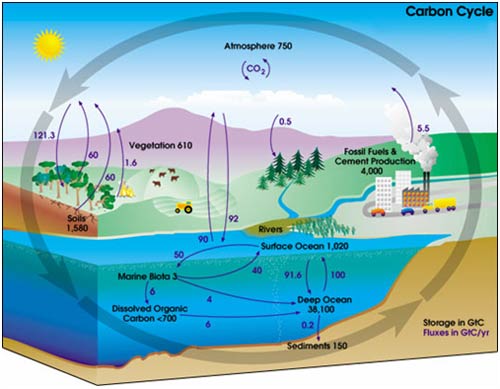
A representation of the carbon cycle (ignore the numbers for now) would look like this one from NASA.

In the IPCC 4th Assessment Report glossary, "lifetime" has several related meanings. The most relevant one is:

“Turnover time (T) (also called global atmospheric lifetime) is the ratio of the mass M of a reservoir (e.g., a gaseous compound in the atmosphere) and the total rate of removal S from the reservoir: T = M / S. For each removal process, separate turnover times can be defined. In soil carbon biology, this is referred to as Mean Residence Time.”

In other words, life time is the average time an individual particle spends in a given box. It is calculated as the size of box (reservoir) divided by the overall rate of flow into (or out of) a box. The IPCC Third Assessment Report 4.1.4 gives more details.

In the carbon cycle diagram above, there are two sets of numbers. The black numbers are the size, in gigatonnes of carbon (GtC), of the box. The purple numbers are the fluxes (or rate of flow) to and from a box in gigatonnes of carbon per year (Gt/y).

A little quick counting shows that about 200 Gt C leaves and enters the atmosphere each year. As a first approximation then, given the reservoir size of 750 Gt, we can work out that the residence time of a given molecule of CO2 is 750 Gt C / 200 Gt C y-1 = about 3-4 years. (However, careful counting up of the sources (supply) and sinks (removal) shows that there is a net imbalance; carbon in the atmosphere is increasing by about 3.3 Gt per year).

It is true that an individual molecule of CO2 has a short residence time in the atmosphere. However, in most cases when a molecule of CO2 leaves the atmosphere it is simply swapping places with one in the ocean. Thus, the warming potential of CO2 has very little to do with the residence time of individual CO2 molecules in the atmosphere.

What really governs the warming potential is how long the extra CO2 remains in the atmosphere. CO2 is essentially chemically inert in the atmosphere and is only removed by biological uptake and by dissolving into the ocean. Biological uptake (with the exception of fossil fuel formation) is carbon neutral: Every tree that grows will eventually die and decompose, thereby releasing CO2. (Yes, there are maybe some gains to be made from reforestation but they are probably minor compared to fossil fuel releases).

Dissolution of CO2 into the oceans is fast but the problem is that the top of the ocean is “getting full” and the bottleneck is thus the transfer of carbon from surface waters to the deep ocean. This transfer largely occurs by the slow ocean basin circulation and turn over (*3). This turnover takes 500-1000ish years. Therefore a time scale for CO2 warming potential out as far as 500 years is entirely reasonable (See IPCC 4th Assessment Report Section 2.10).

Intermediate rebuttal written by Doug Mackie


Update July 2015:

Here is the relevant lecture-video from Denial101x - Making Sense of Climate Science Denial

Last updated on 5 July 2015 by pattimer. View Archives

Printable Version  |  Offline PDF Version  |  Link to this page

Argument Feedback

Please use this form to let us know about suggested updates to this rebuttal.

Update

Updated 'the skeptic argument' on 02/05/2012 to correct formatting errors

Comments

Prev  1  2  3  4  5  6  7  Next

Comments 126 to 150 out of 155:

  1. IanC: Thank you for clarifying. Yes, I had been assuming linearity. None of the statements I had seen (eg "the adjustment time is essentially independent of the residence time") mentioned that they no longer apply if you assume linearity. Dikran M's paper uses linear systems as examples (if I have understood his paper correctly). He uses an example of a wash basin to explain the principle. I worked out the equations that describe it, assuming its outflow is proportional to the volume of water it contains. We have a wash basin, with: * i litres per minute flowing into it. * v(t) litres in the wash basin at time t minutes. * Outflow k v(t) litres per minute. (Note: outflow proportional to v(t) for linearity.) The equation for v(t) is then dv(t)/dt = -k v(t) + i Residence time In equilibrium (ie at t=infinity), dv(t)/dt = 0, so 0 = -k v(infinity) + i so v(infinity)/i= Residence time = 1/k. Adjustment time Consider the wash basin in equilibrium and then, at t = 0, dump an additional D litres of water into it at t = 0. The equation for v(t) is, as before, dv(t)/dt = -k v(t) + i, but with v(0) = D. This has solution v(t) = i/k + D exp (-k t) so the deviation from the equilbrium is d(t) = D exp(-k t) . This means that the adjustment time (ie for the transient to decay to 1/e of its initial value) is 1/k. Adjustment time = 1/k. So it seems that in the case of a linear model, at least one with a 1st order differential equation, residence time = adjustment time. And presumably, with some nonlinear models this may also apply? If you assume finite volume for the ocean, even with a 1st order linear model, the equilibrium changes after the injection of a mass of CO2 into the atmosphere. This means that a proportion of the released CO2 remains in the atmosphere forever (according to the model) - but I think that is different from saying that the residence time and the adjustment time are not equal.
  2. Martin A Indeed in my paper I use a linear model, but it is only a local approximation of the real system. Linearisations of this type are quite common in physics and are good for getting the basic message across, but as I said in the paper it isn't really up to making useful quantative predictions. I think the problem is that you have the outflow being proportional to the volume, however this does not give a reasonable local approximation and you need a linear function of the volume instead (i.e. outflow = k v(t) + C). I think your model is perhaps too simple. This is the principal difference between your model and the one in my paper, so I assume it is where the difference lies. I intitally used a proportional model (as Essenhigh did) but found that if you plot the proportional relationship with the observations it gives an extremely bad approximation, which is why I used linear regression to get a better approximation.
  3. Martin A, One thing that needs to be emphasised is that there is a very big difference between a linear model and a linearised model. If we are dealing with an ODE of the form dX/dt=F(X), saying that it is a linear model means: F(X) is precisely AX+B for all X. A model linearised about (X*) means F(X) ~ C(X-X*) + D for points near X*. Typically X* is chosen to be be an equilibrium point so D is usually 0. 1/A and 1/C give you the adjustment time, but only in the linear model will 1/A give you the resident time as well. The reason is that because the residence time depends on the X and magnitude of the flow, which is explicitly given in the linear model (|AX| and B). On the other hand, information about the absolute magnitude of inflow and outflow is not readily available in a linearised model. It is of course possible that there is some nonlinear F(X) such that upon linearising, 1/C happens to give you the resident time, but unless you know F(X) a priori you cannot assume such a thing.
  4. Dikran M, IanC: Thank you. I need to try and work out some examples for simple models with significant nonlinearity so I can get a feeling for what's really going on.
  5. Dikran, I read Essenhigh's paper, and my impression is that he is using CO2 with C14 to validate his linear model, and then use that as an argument against short adjustment/equilibration time for CO2 in general. Is this a correct interpretation?
  6. IanC Essentially yes. The key point is that C14 is not replenished, so it can only tell you about the residence time not the adjustment time.
  7. Dikran, For the case of C14, the residence time is the same as the adjustment time. I tend to think of the residence time as the time it takes to reduce X to 0, while the adjustment time is the time it takes for X to approach a particular equilibrium. In the case of the C14, the initial perturbation is so large that 0 is effectively the equilibrium, and the data does support a simple exponential decay to 0. In which case the linear model is valid, and the residence time and adjustment time are the same. IMO, the fatal flaw of Essenhigh2009 is that the equilibrium for overall CO2 is very far from 0, so although his model is 'validated' by the C14 data it doesn't actually carry over to the anthropogenic CO2 problem, as it is in a completely different regime!
  8. IanC residence time is the length of time an individual molecule of CO2 stays in the atmosphere, rather than the time it takes to decay to zero. C14 is constantly being generated in the upper atmosphere, so it does have a non-zero equilibrium level. The real problem with Essenhigh's paper is that hea appears unaware of the distinction between residence time and adjustment time. His estimate of residence time is completely uncontraversial, the problem is that a short residence time doesn't mean that anthropogenic emissions are not the cause of the long term rise. The link between residence time and the attribution of the rise in his paper is very tenuous.
  9. Dikran, Sorry what I meant was, the residence time as the time it takes to reduce X to 0 in the absence of a source , which is just X divided by the flux of X out of the box. I believe this is the standard definition of the residence time. To clarify, in 131 are you referring to the residence time and adjustment time of CO2 or C14? I might have misunderstood you.
  10. The non-equivalence of residence and adjustment time evidently depend the system being nonlinear. Is there a reference where a non-chemist can read up on the chemistry of equilibrium between CO2 in seawater and air, to the level of calculating diffusion rates? It seems to be a topic that is: - not simple - somewhat controversial. I'd like to do calculations of my own to understand the nonlinearity.
  11. IanC The adjustment time and residence time in my paper are both for the atmosphere. IIRC there is a preferential uptake of "light" CO2, so C14 would have a slightly longer residence time, but there is so little of it it would have no real effect on atmospheric residence and adjustment times. Martin A No, it doesn't depend on the system being non-linear. The one-box model discussed in my paper is linear, but it has different residence and adjustment times. I don't think the basic physics of ocean uptake is contraversial. Siegenthaler and Sarmiento would be a good place to start. However it would probably be a good idea to reconcile the difference between your model and mine before going on to the oceanic uptake.
  12. Dikran, Ah I see. I originally thought in 131 you are referring to the residence time for C14 and adjustment time for a perturbation of C14, which clearly are the same from the data. I tried explaining this from a more general model, and thought the large initial perturbation will lead to simplifications in the fluxes that will give you this result. Turns out this is unnecessarily complicated: after reading your paper again I realised that your model for the anthropogenic CO2 component can be applied to the C14 data with the addition of a source term, and all the right conclusions follow.
  13. Dikran M: Thank you - I'll go back and look more carefully at your paper. I had thought the examples I had worked out (including the one above) had shown that residence and adjustment times were the same for a 1st order linear system. I think you are quite right. It makes good sense to reconcile your model and mine before introducing any further complications.
  14. Dikran M: I tried to work through your paper but found I was making slow progress. So I decided to reproduce the results of your "A One-Box Model of the Carbon Cycle". Here is my working - I hope I have not made errors despite my tendency to do so. I've made my notation close to yours, though not exactly the same. If you would clarify the points I am sure of (where I've put questions), I'd be very grateful. I am eager to get to the bottom of this (residence time)/(adjustment time) question. Let: C(t) = total atmospheric carbon at time t, (Gt). Fe(t) = Rate that carbon is absorbed by the reservoir from the atmosphere at time t, (Gt yr^-1). This is taken as being given by the formula Fe(t) = ke C(t) + Fe0 where ke = 0.0135 yr^-1 and Fe0 = 182.7 Gt yr^-1 . [Please see question 1 below] Fi = rate that carbon leaves the reservoir and enters the atmosphere, assumed constant and equal to the pre-industrial emission rate, = 190.2 Gt yr^-1 (calculated from values taken from your figure 1). The differential equation for the carbon in the atmosphere is dC(t)/dt = -ke C(t) - Fe0 + Fi = -0.0135 C -182.7 + 190.2 = -0.0135 C + 7.5. [Please see question 2 below] In equilibrium, the carbon in the atmosphere is given by putting dC(t)/dt = 0, which gives Ceq = 7.5 / 0.0135 = 555.5 Gt. The solution for the differential equation, assuming C(0) = Ceq + delta is C(t) = Ceq + delta exp(-ke t). The time constant for this 1st order equation is ke, so the adjustment time is 1/ke = 74.07 yr. [Please see question 3 below] For residence time, your paper talks about carbon of natural and anthropomorphic origin. I did not see why this was necessary. As you say, nature can't distinguish the origin of CO2 molucules so I did not grasp why it is useful to calculate the lifetime of molecules of specific origin. For arbitrary CO2 molecules, the residence time in equilibrium is (content)/(throughput). So residence time = Ceq/Fi = 555.5/190.2 = 2.92 yr. General question on linearity - [Please see question 5 below] Questions 1a. Does "the size of the atmospheric reservoir" (p18) mean the mass of carbon in the atmosphere? 1b. How are the numbers for (Fi - Fe) calculated, please, (in enough detail I can calculate them myself from the Mauna Loa or other data)? 2. This involves taking differences of largish numbers which I imagine are not precisely known, to get smallish differences. An error of a few percent in the numbers would mean that their difference contained no useful information. Is there reason to believe the difference has meaning? 3. This is slightly different from your value of 74.2 yr - I assume this is a typo. 4. Have I got the residence time right (for CO2 of arbitrary origin)? Or can you help me understand why calculating the residence time of a subset of CO2 molecules is useful? 5. Linearity. In ES09, Fe was given by Fe = ke C. You have replaced this with a function Fe = f(C) where f(C) = ke C + Fe0. This function is the formula for a straight line but that does not make the equation linear, so far as I can see. For the equation dC(t)/dt = f(C) to be linear, the function f(".") must satisfy f(C1 + C2) = f(C1) + f(C2) for any C1, C2, because this is how linearity is defined. In this case, for example f(0 + 0) = f(0) = Fe0. But f(0) + f(0) = 2Fe0. So it does not, so far as I can see, qualify as a linear differential equation. Does this make sense? Have I missed something? Thank you your help.
  15. Hi Martin, I'm sorry I haven't replied to your email yet (exam time here, only just finished my marking). I'm about to go home now, so I'll try and answer a few quick points now and will be back tomorrow. 1a. yes, the atmospheric reservoir is just the mass of carbon in the atmosphere. 1b. (Fi - Fe) is calculated via the mass balance argument (conservation of mass implies that it is the same as dC - anthropogenic emissions). So if you download the mauna loa dataset and the emissions (fossile fuels and land use change, you should be able to reproduce figure 6, which I used to calibrate the model). 2. The data for dC and anthro emissions are known with good certainty, so while Fi and Fe are uncertain, the difference between them is constrained by the uncertainty on dC and anthro emissions. I doubt the error from this source has a greater effect on the results than the crudeness of the model, which is only the simplest possible approximation. As I said in the paper it isn't of any use for quantative predictions, only for getting a qualitative understanding of the very basics. 3. or rounding somewhere. 4. I think that residence time would be for pre-industrial conditions, rather that todays, as we have increased the atmospheric reservoir above its equilibrium value (and the uptake will have increased a bit as well). The residence time (for a given isotope) is the same regardless of its origin. The important point is to explain why there is very little "anthropogenic" CO2 in the excess above the equilibrium concentration, which is because it gets replced by "natural" CO2. The residence time is really the time an individual molecule stays in the atmosphere on average, so it is really only properly defined in terms of a subset of one molecule. Sorry, have to dash now, my lift home has arrived! Hope this helps.
  16. Dikran M: Commiserations on the exam marking - I can't imagine it's much fun. Thank you for the comments - I'll study them carefully and try to do some calculations with the data. I came across the paper H. Rodhe + A Björkström "Some consequences of non-proportionality between fluxes and reservoir contents in natural systems" (Tellus(1979),31, 269-278) which specifically studies nonlinear equilibrium. It reinforces my conjecture that nonlinearity is necessary for (residence)/(adjustment)< 1.
  17. Martin, Abell & Braselton ("Modern Differential Equations", Saunders College Publishing, 1996) on page 72, say that a first order linear d.e. can be written in the form dy/dx + p(x)y = q(x) The d.e. defining the one-box model in my paper dC/dt = F_i^0 - k_eC - F_e^0 is of that form, where y = C x = t p(x) = k_e = constant q(x) = F_i^0 - F_e^0 = constant As the one box model exhibits an adjustment time that it much longer than its residence time, but is described by a linear d.e., then AFAICS this establishes that the conjecture is false. Non-linearity is not required for the adjustment time to be longer than the residence time.
  18. DM: Yes, thank you, you are right, nonlinearity is not required for (adjustment time)>(residence time) for your model. I guess that your model, though linear itself, approximates a nonlinear relation between the atmospheric CO2 concentration and rate of diffusion from atmosphere to environment better than the linear relation assumed in ES09. I think I should have said that for (adjustment time) > (residence time) then dC/dt cannot be directly proportional to C ie if you have dC/dt = const.V + F_i then you will get (adjustment time)=(residence time). I'm working on using the Mauna Loa data to reproduce your result and to get an understanding of why your model is a better representation of reality than ES09.
  19. And like a bad penny, this silly argument has risen again. Someone named Gosta Petterson (a professor emeritus of biochemistry and specialist in reaction kinetics, not atmosphere or carbon cycle) is once again claiming that individual molecular residence time (one way) is somehow identical to CO2 concentration change time (with most CO2 molecules simply exchanging for another from a different climate compartment), a much slower process. 

    There's a good discussion of this topic and the errors involved on SkS, under The Independence of Global Warming on Residence Time of CO2.

    Sadly, this appears to be yet another example of an emeritus professor wandering out of his specialty, and with little perspective proclaiming an entire field of science invalid. And of long-debunked myths being recycled over and over again...

  20. "Biological uptake (with the exception of fossil fuel formation) is carbon neutral: Every tree that grows will eventually die and decompose, thereby releasing CO2. "

    I can see how that would be true for the portion of a tree above ground (assuming the wood isn't used to make a house or something that locks up the wood for 100+ years), but my impression is that the roots are probably as large a carbon sink as the above ground tree and that the smallest tendrils will constantly grow and die back and essentially become part of the soil, fixing their carbon for a long time. Do you have a paper that supports your assertion that trees/plants are carbon neutral? (Preferably one that actually measures the carbon fixing of below ground material over time.) It seems unlikely to be carbon neutral. 

    This paper argues that organic carbon stored in forest soils are a reservoir roughly the same size as the atmosphere, so we aren't talking about a small effect. http://www.dpi.nsw.gov.au/__data/assets/pdf_file/0006/389859/Principles-and-Processes-of-Carbon-Sequestration-by-Trees.pdf

  21. Ashby, there are fungi and bacteria in the soil that break down the roots of dead trees as well.  I suspect how fast this happens depends on the moisture and oxygen availability.  If this were not true, we would be digging up the roots of dead trees everytime we dig a hole in the ground, which is not the case.

  22. Ashby @145, according to Melin et al (2009), root systems apparently account for only 20% of the biomass of a tree (citing Hakilla, 1989).  Further, for Norway Spruce, 4.6% of the subterainian biomass decomposes per year, so that 50% is lost in 15 years, and 95% in 64 years.  That is faster than the 3.8% of soil carbon respired to the atmosphere each year (see diagram in main article), but not sufficiently so as to expect a large increase in the soil reservoir from reforestation relative to the increase in the vegetation reservoir from the growth of the trees.

  23. Below-surface carbon in forest can be quite complex. I say "below-surface" because there is not only roots, but also carbon in other soil micro-organisms, plus carbon from decaying roots, etc., as well as the carbon that is carried into the soil from surface litter and such.

    Roots do decay over periods of years to centuries, depending on size (and what forect type you are talking about). Tree trunks and branches fall to the forest floor, and then slowly rot - but the more persistent carbon compounds produced will work their way into the soil.

    In tropical forests, soil carbon and surface litter are rapidly decayed, so soil carbon content is low - root mass will be the dominant store. In the boreal forest, soild carbon often exceeds (per hectare) the carbon stored in trees above ground, due to cooler temperatures and slow decay rates.

    Fire obviously returns carbon rapidly back to the atmosphere, as biomass is burned. Removal of above-ground mass (burning, logging, etc.) will often lead to a rapid drop in soil carbon, as the soil is exposed to sunlight and warmer temperatures. The loss of soil carbon often exceeds the uptake by new growth, so a rapidly-growing forest in a recently-disturbed area can still be a source of carbon (loss to atmosphere), not a sink.

    Turning lumber into houses and such does represent a moderate-term carbon sink. Carbon budget models of the forest will account for these factors, such as the Canadian Carbon Budget Model.

    I'm most familiar with the dynamics of boreal forests. One major study from 20 years ago was the BOREAS project. A Google search for "BOREAS soil carbon" gives megahits.

    Forests do represent major carbon storage, and that is where some of the carbon from burning fossil fuels is going, but by and large they do not represent a long-term permanent sink.

  24. Hi, the question I have is how do we know that global CO2 emissions weren't increasing at a rate of 3.3x back before the industrial revolution? (Sorry forgot the units). If so, how did the process of figuring that out work? 

    Thank you. 

    Response:

    [Rob P] - There are multiple lines of evidence, but the simplest to understand is that tiny bubbles of air are trapped in snow on the giant ice sheets of Antarctica and Greenland. As this snow is slowly compacted to form ice, the air trapped inside is sealed off from the atmosphere. The ice that has survived for hundreds of thousands of years is therefore a continuous record of the Earth's atmosphere. Core samples are obtained by drilling down into the ice with specialized drilling rigs, and the ice core is later painstakingly analyzed to determine atmospheric CO2 concentration.

    Consider the last 10,000 years for instance.......


    Tom Curtis' Climate Change Cluedo is also a worthwhile read if you want to learn more.

  25. Zadams @149, I assume you are asking how do we know that atmospheric CO2 was not increasing by 3.3 Gigatonnes of Carbon per annum  (1.56 ppmv) prior to the industrial revolution? 

    Well, to start with, the increase in CO2 concentration observed at Hawaii shows an accelerating trend:

    Decade Total Increases Average Annual Rates of Increase
    2005 – 2014 21.06 ppm 2.11 ppm per year (4.47 GtC per year)
    1995 – 2004 18.67 ppm 1.87 ppm per year (3.96 GtC per year)
    1985 – 1994 14.24 ppm 1.42 ppm per year (3.01 GtC per year)
    1975 – 1984 14.40 ppm 1.44 ppm per year (3.05 GtC per year)
    1965 – 1974 10.56 ppm 1.06 ppm per year (2.25 GtC per year)
    1960 – 1964 3.65 ppm 0.73 ppm per year (5 years only) (1.55 GtC per year)

    Second, CO2 data from icecores, and C13 data from icecores, speliothems, corals, and mollusc shells show CO2 levels to have been near constant prior to 1750 going as far back as the end of the last glacial.  I discuss these in a post here that canvasses the wide range of evidence showing the recent increase in CO2 to have been anthropogenic (see in particular points 1, 5 and 10).

    However, the most fundamental reason is arithmetic.  The atmosphere currently has about 400 ppmv of CO2 (848 GtC).  If atmospheric CO2 had been increasing continuously by 3.3 GtC per annum into the past, just 257 years ago, the atmosphere would have had no CO2 (at which point there could be no photosynthesis, and hence no plants on which we live).  Even an increase of as little as 0.09 GtC per year would mean that at the start of the phanerozoic, at the time humans were inventing agriculture, there would have been no CO2 and hence no possibility of our wheat, rye, rice or maize growing.  So, even if we had no CO2 records going back into the past, we would know that the current rate of increase is much greater than fifty times the long term average rate of increase leading into the industrial revolution.

    So, if we want to believe that the increase in CO2 is natural in origin, we need to believe that just as the industrial revolution kicked of, the long term natural rate of net emissions suddenlty increased by a factor of 10 or more, and then continued to increase over the following 250 years in almost perfect sync with know human emissions until they rose to their current level of well over fifty times the previous long term rate of increase.  Further, at the same time we have to believe their is an independent natural sink that did not previously operated that increased at the same rate as human emissions to nullify them, and which is triggered by those emissions so that it should not be included in the net natural emissions, is also incapable of stabilizing net natural emissions (which on this scenario are anything but stable).  Put simply, that is not an elegant hypothesis.

    Finally, FYI, from icecore data we know that the long term increase in CO2 over the holocene up to the industrial revolution was actually about 0.004 GtC per annum; and there is good reason to think that most of that was driven by deforestation driven by the expansion of agriculture (ie, that it was anthropogenic).

Prev  1  2  3  4  5  6  7  Next

Post a Comment

Political, off-topic or ad hominem comments will be deleted. Comments Policy...

You need to be logged in to post a comment. Login via the left margin or if you're new, register here.

Link to this page


The Consensus Project Website

THE ESCALATOR

(free to republish)


© Copyright 2024 John Cook
Home | Translations | About Us | Privacy | Contact Us