Climate Science Glossary

Term Lookup

Enter a term in the search box to find its definition.

Settings

Use the controls in the far right panel to increase or decrease the number of terms automatically displayed (or to completely turn that feature off).

Term Lookup

Settings


All IPCC definitions taken from Climate Change 2007: The Physical Science Basis. Working Group I Contribution to the Fourth Assessment Report of the Intergovernmental Panel on Climate Change, Annex I, Glossary, pp. 941-954. Cambridge University Press.

Home Arguments Software Resources Comments The Consensus Project Translations About Support

Bluesky Facebook LinkedIn Mastodon MeWe

Twitter YouTube RSS Posts RSS Comments Email Subscribe


Climate's changed before
It's the sun
It's not bad
There is no consensus
It's cooling
Models are unreliable
Temp record is unreliable
Animals and plants can adapt
It hasn't warmed since 1998
Antarctica is gaining ice
View All Arguments...


Username
Password
New? Register here
Forgot your password?

Latest Posts

Archives

Astronomical cycles

Posted on 17 June 2010 by Riccardo

Guest post by Riccardo

Recently a new paper by Scafetta came out (a freely downloadable version can be found on arxiv but I don't know if they are exactly the same). In a few words, Scafetta connect the orbital motion of the planets with solar variability and hence on earth climate. He found a dominant 60 years cycle which, he claims, greatly downplay the anthropogenic contribution to the warming after the '70s. I won't go through the details of his analysis and the hypothesis on the yet to be discovered physical mechanism behind. Forget about physics for a moment, as Scafetta does, and think only about cycles and periods.

He does a nice and fascinating analysis of various orbital cycles which cause the motion of the sun around the center of mass of the solar system. It's assumed that in one way or another the gravitational pull affect sun activity. He then compares the power spectra from detrended Hadley's temperature data with that of the orbital cycles and obtains the nice graph reproduced below.


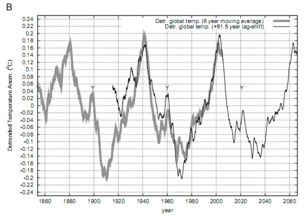
Fig.1: reproduction of fig. 10B in the original paper. It shows the eight years moving average of the temperature anomaly detrended of its quadratic fit (gray); the thin black line is the same curve shifted by 61.5 years.

The data has been detrended assuming an underlying parabolic trend. The main 60 year cycle, due to the alignment of Jupiter and Saturn, shows up very clear, but there are more. In particular, he identifies a total of 10 cycles due to combination of planets motion and one due to the moon (fig. 6B in the paper). Of those cycles, only two more are considered significant, namely those with periods of 20 and 30 years.

Fascinating. But then, a few pages later, Scafetta writes:

However, the meaning of the quadratic fit forecast should not be mistaken: indeed, alternative fitting functions can be adopted, they would equally well fit the data from 1850 to 2009 but may diverge during the 21st century.

His warning is on the problem of extrapolation of the trend in the future, which he nonetheless shows. But this sentence made me think that it's true, once we put physics aside, we're free to use the trend we like; so why parabolic?  I decided to take a closer look, and this turns out to be the begining of the end.

The first and more obvious try is a linear trend and then one with a higher power. I kept the functional form y=a(x-1850)n-b used by Scafetta, but let n be 1,2 or 4. Here's what I got.


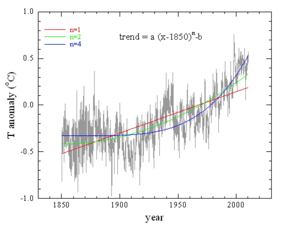
Fig.2: HadCRUT3 monthly data (grey) and the fits for n=1 (red), 2 (green) and 4 (blue).

Already by eye inspection it may be noticed that, due to the different curvature of the fitting functions, the behaviour is different between the middle and the extremes of the range. To be quantitative, we need to calculate the residuals, i.e. the difference between the data and the trends.

The fits were performed using the raw monthly data, as shown in fig. 2, but given that we are looking for long term cycles, I smoothed the data before detrending to clean them up a bit, as Scafetta did too. The results are shown in the following figure.


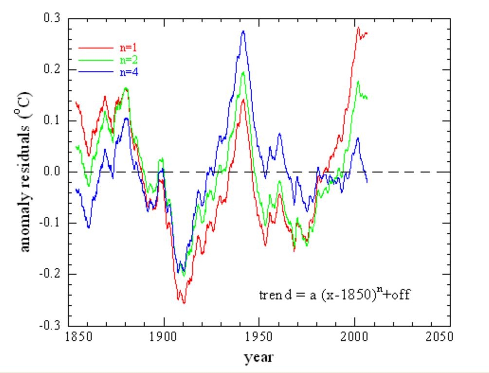
Fig.3: residuals calculated with the trend curve shown with n=1 (red), 2 (green) and 4 (blue).

As noted before, the behaviour at the extremes of the range is opposite with respect to that at the center and the two peaks at year 1880 and 2000 get smaller on increasing n. In particular, for n=1 the curve barely flattens aroud year 2000 while for n=4 only a small short-lasting peak is left. Only with n=2 we get the three nice equal amplitude peaks.

More generally, for n=4 the claimed 60 year cycle seems to vanish after the peak at year 1940. It's not to say that the n=4 trend has more value than the n=2, but in the end we can say that the nice cyclic behaviour seen in fig. 1 depends on the choice of the trend function. It's worth to recall that its choice is arbitrary, no physics behind it.

I tested this findings with the other global surface temperature datasets (GISS and NCDC) and, not unexpectedly, they confirmed. The claim that the anthropogenic contribution to the increase in temperature after the 70s has been overestimated has then to be dismissed, at least until we can make a proper choice of the underlying trend.

Still, small, periodic and short-lasting peaks seem to be real. More accurate and hopefully physics-based studies on decadal variability are required, taking into account all possible internal and external contributions.

0 0

Printable Version  |  Link to this page

Comments

Prev  1  2  3  

Comments 101 to 141 out of 141:

  1. There appears to be an 'Article in Press' version of the Scafetta paper over at SPPI The fact that SPPI [of Monckton infamy] received what was probably an embargoed pre-publication copy could easily lead one to draw all manner of conclusions about the motives behind this. Scafetta has produced [ahem] poor weak papers in the past and I suspect this attempt is just more of the same.
    0 0
  2. Looking back at the 100% AGW 1970-2000 IPCC claim, I noticed a discrepancy. On page 1 he states "practically" 100%, but on pages 9 & 13 he leaves the word "practically" out. Isn't that something the reviewers should catch?
    0 0
  3. Skeptical Science-Scafetta Enough already. It's elementary math and statistics that fitting a function to the data is only valid for the extent of the data. The fitted curve cannot be used to extrapolate future values. A good example are some of the IPCC graphs attempting to estimate future values of the temperature, depending on various emissions scenarios. In order to fit the 'curve" some of the emissions scenarios imply that temperatures in the past would be a hundred or more degrees below 0. For scientific usage, fitting a curve might show that the data has some periodic function in it, prompting a search for possible mechanisms, or it might give some insight into possible mechanisms to investigate. That, despite some of the exaggerated claims, is the whole point of the Scaffeta paper. There are apparent periodicities in the temperature data which coincide with periodicities in various solar, lunar, and planetary orbits. That suggests there might be a causative relationship that should be investigated. Very similar to the idea that rising C02 levels, even though they follow the intial temperature rise, correlate to rising temperatures in a fashion and might be part of the cause of rising temperatures, rather than an effect of them. the same thinking applies to any paramaterized model(all the GCM models in use). As pointed out by many others, any model with adjustable parameters in it is one person's opinion about what is going on. It may be useful in suggesting areas for further study and data gathering, it may suggest further experiments, but the model itself is useless for prediction outside the range of data used to calibrate it. For a good example of a non-parametric model look into the photo electric effect. A nice, simple equation, from first principles, that gives valid results over a wide range.
    0 0
  4. philc - I dont believe you understand how parameterisation is done in GCMs. faq II for even more detail. In particular, I object that the "adjustable parameters" in GCM can be tuned in the way you say. Lets say that I use fundamental physics to create full model of process. It can be used over entire range of observable data. However, it might be also impossible to use in full form from computation limits in GCM or because if scale. You can however replace with parameterized model that is easy to calculate but which you can nonetheless verify works over full range. I suggest further discussion goes in "are models reliable" rather than here.
    0 0
    Moderator Response: scaddenp's suggestion that further discussion happen on the Models are unreliable thread is a good one. So please do.
  5. Chris #100 I have not had time to go back to the prior sea level discussion, being away for a few days. It should be noted however that the very fact that there was an 'apparent' slowdown of the rise in the 2006-2008 period observed by Jason, followed by an impossible 6.5 mm/year to date; does indicate an unexplained variability in either the sea level or the Jason measurement. We are talking global sea level rise jumping from around 2mm to 6.5mm per year. This is a huge burst of heat equivalent; entirely incompatible with the steadily increasing imbalance proposed by CO2GHG theory. It would imply a thermal expansion rise of 3-4mm/year which is equivalent of about 280E20 Joules/year which is double Dr Trenberth's 145E20 Joules /year 'observed' by his 0.9W/sq.m TOA imbalance. Explaining this a noisy data might be credible if it applied to a part of the biosphere where the sum of the other parts even themselves out; but it is scarcely credible globally; for the whole of the planet.
    0 0
  6. Ken Lambert at 23:50 PM on 28 June, 2010 Well yes Ken, that's the point. You chose to make a great deal out of an apparent slow down in sea level rise. My point is that one cannot make profound interpretations from a very short period of data. After all if you wish to assert that the apparent slow down is significant then you can't really choose to ignore an equivalent apparent speed-up in sea level rise. We don't know to what extent these apparent slow downs and rises are fully real (they’re certainly at least partly real; see below). Overall the data continue to be compatible with a continuing trend in sea level equivalent to a rise somewhat above 3 mm.yr-1. This is wrong: "...entirely incompatible with the steadily increasing imbalance proposed by CO2GHG theory. If by "CO2GHG theory" you mean the rather well-founded expectation that the earth surface temperature will rise under the influence of a radiative imbalance towards a new equilibrium temperature around which it will fluctuate as a result of natural variability (i.e. the theory of enhanced greenhouse forcing), there isn't anything necessarily incompatible with the observed sea level rise data. It would be a fundamental misunderstanding to think that there should be anything necessarily "steady" about the progression of manifestations of radiative imbalance particularly when assessed over short periods. One needs to consider: (i) measurement errors. These are smaller for sea level rise measurements than for ocean heat content (OHC) measures, but they are significant as is obvious from inspection of the data . This is always a good reason for preferring longer term trends over very short time periods. (ii) real short term variability. This is likely to be large [*]. And of course we know this from simple inspection of the data. Natural variability will enhance the apparent greenhouse-forced sea level rise during some periods (El Nino, solar cycle, reduced albedo), and during other periods suppress the apparent sea level rise (La Nina, solar cycle, enhanced albedo, volcanic activity). Overall this natural variability will more or less reduce to near-zero with respect to trends. Therefore if we wish to make profound interpretations about trends, we obviously choose to assess the progression of parameters over longish periods in which this variability is averaged out. [*] For example, the redistribution of ocean heat during El Ninos and La Ninas can have very large temporary effects on sea level. It’s not unheard of the have a short term (year or so) rise of 10-15 mm.yr-1 during strong El Ninos, and largish sea level decreases during La Ninas. It’s dumb to pretend that these effects don’t occur, or to ignore them when attempting fundamental interpretations about responses to radiative imbalances.
    0 0
  7. Ken Lambert at 23:50 PM on 28 June, 2010 Sorry to plug this again. Have a look here to see the updated satellite record with the global seasonal variations retained, and further down the comments there's a chart showing SH/NH seasonal variations. The annual rate of rise/fall easily exceeds your figures. It's the overall trends we're talking about. Jason 1 had some issues, not sure if they're fixed. Jason 2 and Envisat are current.
    0 0
  8. KL #105
    This is a huge burst of heat equivalent; entirely incompatible with the steadily increasing imbalance proposed by CO2GHG theory.
    The myth of a monotonic increase is a frequent climate contrarian talking point. The theory has no such requirement. Perhaps this is one for the common arguments page, although the idea that noise exceeds signal over short time periods is so obvious to everyone except the so called sceptics, that it's an argument that's trivial to rebut.
    0 0
  9. Further to kdkd's comment to Ken, here's an extended quote from a blog post by Michael Tobis I think talks to the whole matter behind this thread, that is to say whether some external influence is going to nullify unrelated processes here on Earth. There is some implication that there is an "AGW theory" and that there is an argument in its support, and that said argument is a cohesive thread starting with Fourier and ending at the dreaded-extremist-boogeyman-Gore, and that failure of any chain in said argument necessarily implies "see, so no carbon policy is necessary". (I'm missing a few steps in their reasoning here, too, but that's another topic still.) I claim there is no "AGW theory" in the sense that there is an argument that four colors suffice, or more fairly, that stars follow an evolutionary path based on their mass. AGW is not an organizing principle of climate theory at all. Hypotheses, organizing principles, of this sort emerge from the fabric of a science as a consequence of a search for unifying principles. The organizing principles of climatology come from various threads, but I'd mention the oceanographic syntheses of Sverdrup and Stommel, the atmospheric syntheses of Charney and Lorenz, paleoclimatological studies from ice and mud core field work, and computational work starting with no less than Johnny von Neumann. The expectation of AGW does not organize this work. It emerges from this work. It's not a theory, it's a consequence of the theory. Admittedly it's a pretty important consequence, and that's why the governments of the world have tried to sort out what the science says with the IPCC and its predecessors. That tends to color which work gets done and which doesn't, and I think it should. As Andy Revkin pointed out, it may be time to move toward a service-oriented climatology, or what I have called applied climatology. The point is that this amounts to application of a theory that emerged and reached mathematical and conceptual maturity entirely independent of worry about climate change. So attacks on climate change as if it were a "theory" make very little sense. Greenhouse gas accumulation is a fact. Radiative properties of greenhouse gases are factual. The climate is not going to stay the same. It can't stay the same. Staying the same would violate physics; specifically it would violate the law of energy conservation. Something has to change. For a little more on what must change, how much, etc. see the rest of Tobis' post. My point in quoting Tobis is to make a helpful reminder that "falsifying" the notion of anthropogenic global warming would require an upheaval of research none of us are going to witness. So don't look to external matters such as the moon and stars or things that make graphs wiggle to put a neat "done" on the matter.
    0 0
  10. Chris#106 kdkd#108 Well no, Chris. The core of CO2GHG theory is a simple IPCC equation: F.CO2 = 5.35ln(CO2b/CO2a)W/sq.m where CO2a is the pre-indistrial CO2 concentration (280ppmv)and CO2b is the current concentration. This is logarithmic and monotonic. Every year the radiative energy flux imbalance F.CO2 increases with CO2 concentration. The argument that global 'noise' seriously distorts this heat accumulation assumes some sort of storage mechanism (where else but the oceans?), which can store heat and release it in noisy bursts globally. OHC in the top 700m has been flat for 6 years. Seems inconsistent with anything but a flattening sea level. Peter Hogarth #107 Had a good look at "Visual Depictions of Sea level Rise" and links from March10. Please explain the trend lines for the deployment of Jason 2 and Envisat. I am seeing Jason 1 with a linear trend for the last 8 years of about 2.1mm/year and an offset of 4-6mm at the start of the TOPEX-Jason transition in 2002 from here: http://sealevel.colorado.edu/current/sl_ib_ns_global.jpg
    0 0
  11. Ken Lambert at 00:32 AM on 30 June, 2010 Are you looking at the image or the actual data? From JASON 1 data 2002 up to end 2009 I get a trend of 2.61 mm/year, inverse barometer applied, seasonal signals retained. Adding GIA corrections would add another 0.4mm (current estimate) as in the chart you refer to. JASON 2 has obviously not had enough time (2 years) to develop a meaningful trend of its own as yet but the high accuracy and successful calibration means that the data points can be added to the overall picture. I suspect this is what the final points are on the Colorado chart (ie Jason 2) but I will check. Envisat has been going since 2002 as with Jason 1, and TOPEX continues through to end 2005 so there is overlap rather than the step transition you imply. There are also a couple of other satellite altimeters which add to our knowledge. The chart I presented has an unweighted composite of all data, but you can check on several official sites for similar charts. I haven't looked at the data for a couple of months, I'll check and let you know if I find any surprises.
    0 0
  12. Ken #110 The main flaw in your argument is that you assume a perfect measurement model through space, time and instrumental precision. As none of these conditions are met, your entire argument is invalid.
    0 0
  13. Peter Hogarth #111 I used this chart: http://sealevel.colorado.edu/current/sl_ib_ns_global.jpg which is IPB corrected and seasonal signals removed. Running a linear fit between 2003 and 2009 gives about 2.1mm/year and 2002 to 2010 gives about 2.4mm/yr. It is clear that the 3.0 +/- 0.4mm/year linear trendline is not a good match for the 2002 - 2009 period of Jason 1. The 60 day smoothed line is above the trend for the 2002-2007 period and crosses below it for 2007-2010, with an uptick in the last year or so apparently due to Jason 2. This is clearly a flatter trend for the Jason 1 perod than the 17 year trend line. It sounds like splitting hairs, but according to Dr Trenberth's Table 1 (Aug09 paper 'Tracking Earth's global energy') the total land ice loss accounts for about 2.0mm/year of SLR but only 2-3E20 Joules of heat is required to melt it, while every 0.4 - 1.2mm of thermosteric rise equals about 20-95E20 Joules of increased OHC. So finding more steric rise is the only way to get closer to an energy balance; and more ice melt rise rapidly worsens this energy budget shortfall. Problem is you can't have increased glacier melts and a flattening SLR without reducing the steric component consistent with a flat OHC in the top 700m; and have a TOA energy imbalance of 145E20 Joules/year at the same time. It is indeed a travesty of conflicting data.
    0 0
  14. Ken Lambert at 00:37 AM on 1 July, 2010 I've downloaded the latest Colorado data. The original full series for all satellites are netcdf format from other sources, but I'll have to wait until I get to work to download that and double check. If you look at the Colorado website there's a section on updates. There was a problem (as I indicated) with Jason 1. I suspect that either Jason2 data has been spliced or has been merged from 2008 in the data you have, making your trends a little dubious, The 2.61 mm/yr trend I indicated is from "pure" (corrected) Jason 1 data. I will check as my last full download was a couple of months back. Anyway, I would gently suggest that the data variability (I have also seen the raw data!) means that we have to average all of the data available to allow our trend to be as robust as possible (statistically), rather than try to make mini-trends of sub-sections and draw conclusions, the +/-0.4mm/year error is only valid over the entire time series. If I include all satellite data our confidence in the result should increase. Try putting 2 sigma error bars on your data? I don't think "flattening" SLR or "conflicting data" is supportable here.
    0 0
  15. Ken #113 Again I refer you to my response #108. Your continued ignoring of this inconvenient truth (that the measurements are insufficiently precise over very short time periods rendering your argument invalid) appears to demonstrate that you're mainly interested in hiding under a cloud of technical sounding rhetoric. Anyway, doesn't this discussion live in the sea level rise thread?
    0 0
  16. re 104 scadenp: Guess you missed the point. Scafetta's model is fitting a curve to the data. Intrinsically, the model cannot be guaranteed to work outside the range of the data. The only way it might work is if the functions chosen for the fit actually happened to be functions that were actually good descriptions of the underlying processes. In Scafetta's paper this may actually be the case, since he is using functions drawn from the data and not unreasonably extrapolating that they might continue to describe the data into the future. While the exact mechanism that might cause the climate to respond to the motions of the planets/sun/moon are not known, it is quite reasonable to assume that the mechanism is unlikely to suddenly change or that the motions of the planets are going to vary unpredictably. The mention of climate models was not the point, but just to emphasize that curve fitting is a very iffy way to make predictions.
    0 0
  17. kdkd #115 It seems that the 17 year record is a splicing together of a chain of 3 satelite records (TOPEX, Jason1, Jason2) with differing accuracies and precisions. This chain is only as good as its weakest link. If short links are involved (ie Jason 2) then they should probably be deleted from the composite to give a consistent year on year record. Confine your comments to these technical issues rather than judgements of truth or untruth.
    0 0
  18. Ken Lambert at 00:32 AM on 30 June, 2010 Ken Lambert at 00:33 AM on 2 July 2010 Ken, I suggest that you really need to find a way to address these issues with a little more scientific rigour. You were shown in some detail the manner in which the Topex and Jason data were merged here. Yet you continue to make unscientific and unsupported assertions about "offsets", and other unsubstantiated judgemental statements about the data. You are pushing your prejudices far too hard over this issue; kdkd is quite right to keep pointing this out. The bottom line is that the current sea level is pretty much smack on the level that one would have predicted 17 years ago by extrapolating forward in time with a rise somewhat above 3 mm.yr-1 as simple analysis of the data shows (dispassionate readers should also read Peter Hogarths nice description ). Your continued misunderstanding of the nature of the Earth response to enhanced greenhouse gas concentrations isn't helping you. Incrementally increased [CO2] doesn't necessarily equate to incrementally increased TOA radiative forcing, and neither of these (incrementally increasing [CO2]; incrementally increased forcing) necessarily result in incremental changes in the parameters (like sea level rise) of the Earth/climate response. That is so obvious as to be trivial. The TOA radiative forcing waxes and wanes as contributions from natural variability (solar; volcanic; clouds; albedo) modulates the greenhouse-induced forcing. In addition to these contributions, natural variability affects specific parameters of the Earth response. So sea level rise responds both to the variability in TOA forcing, as well to specific factors related to the temporal distribution of ocean heat that enhances and decreases the progression of sea level rise (e.g. during El Nino and La Nina events). Because the temporal progression of Earth responses to enhanced greenhouse gas is poorly predictable, both in its general trend and due to this natural variability, the effect of enhanced greenhouse forcing on the Earth system is normally assessed in relation to the surface equilibrium temperature response, once the climate system has re-equilibrated with the forcing. "CO2GHG theory" (as you call it!) has rather little to say about the exact progression of climate-related parameters (like sea level) other than that these will fluctuate around the trend on the progression towards equilibrium. It is a total fallacy (and a strawman argument) to think that one should observe continuously incremental changes in any parameter of the climate system, as the latter progresses to a new equilibrium state.
    0 0
  19. Chris #118 Just stick to the numbers Chris, and refrain from your own judgmental terms such as 'prejudices, unscientific, unsupported assertions etc etc' with regard to my arguments. I am simply pointing out that if you want to reduce the analysis to linear trend lines, then doing this for different satellites sliced together is quite consistent with that approach; and if you do that you get an offset. The offset disappears it the trends are not linearized. Why do these SLR charts have to be fitted to linear trend lines in any case? BP showed that the Colorado Chart here: http://www.skepticalscience.com/news.php?p=2&t=89&&n=150 Post #82 "I have calculated least square fit quadratic. It turns out sea level rise is actually decelerating in this 16 years long period. Acceleration term is -0.108 mm/y2." Prove to me that BP's quadratic approach is wrong! Let's have a look at steric rise - it does not seem to be linear with the OHC increase either. Dr Trenberth quotes a range of 0.4mm steric SLR equalling 20E20 Joules and 1.2mm equalling 95E20 Joules. This is 50E20 Joules/mm at the bottom and 79E20 Joules/mm at the top of the range. Nature tends to be rather non-linear. As you know CO2 forcing is logarithmic and radiative cooling by S-B is exponential (T^4). Claims that most of the SLR is steric are not supported in Dr Trenberth's paper viz. 2mm land ice melt and 2.5mm 'observed' - leaving only 0.5 mm steric. You have not addressed the point that you can't have a high ice melt component of SLR and a high steric component at the same time and meet the 'observed' SLR; and even worse - the global energy budget shortfall gets rapidly larger with an increasing ice melt portion because a 1mm of SLR from ice melt needs only about 1.5E20 Joules, and 1mm of steric rise needs 50-79E20 Joules. Please explain this problem; keeping in mind that the CO2GHG theory requires that the biosphere gain 145E20 Joules/year every year and increasing each year (bar the occasional volcano, or dimming sun or increased clouds - both the latter (sun and clouds)are reputedly well constrained and accurately known NOT to be offsetting CO2GHG warming).
    0 0
  20. Ken #119 BP would need to present regression diagnostics to show the validity of his quadratic fit compared to a linear fit. As it stands he presents too little information to assess its validity. My impression is that there's nothing to choose between a linear or quadratic fit, but I'd like to see the AKI statistic for each fit before making a definitive conclusion Your approach is profoundly unscientific anyway - you hide behind a spray of semi-technical meanderings. here is yet another explanation of why your approach lacks validity.
    0 0
  21. I downloaded BP's data that he used for the "quadratic fit", and without further information it's impossible comment on the validity of what he did, apart from noting that looking at the regression diagnostics for a linear fit, there are few questions about the validity of the linear regression, and I'd question the need to use an alternative approach.
    0 0
  22. Ken Lambert at 00:24 AM on 3 July, 2010 ONE offsets: You're trolling Ken. We've already shown you how the satellite data was merged to effectively eliminate offsets. You ignored this, but you should address it if you wish to pursue the insinuation of "offsets". I have asked you and kdkd has asked you to show how you determined the offsets. You ignored those requests too. I suggested what you might have done based on your assertions. You ignored that. And yet here you are asserting "offsets" by insinuation again. That's trolling. Why not simply state explicitly how you determined these apparent "offsets"? I think I know what you've done...if so it's invalid numerology. But we won't know for sure unless you tell us. TWO: linear/quadratic trends: Science isn't addressed by attempts at bullying Ken ("Prove to me that BP's quadratic approach is wrong!"). Fitting a quadratic to a temporal progression of a parameter is meaningless unless one has some independent justification for the quadratic and its particular form, and you should be careful not to be fooled by flawed analyses [*]. In the case of a relative short (18 year) period of sea level rise with significant variability from measurement "noise" and internal variability we have to be careful not to mislead ourselves with inappropriate curve fitting that is hopelessly biased by the short term variability (see [*] below). However we can ask a simple question about the data, namely: ” Given the variability in the data is the sea level rise consistent with a linear progression in time, or is it accelerating or decelerating?” If we take the data (say the unadjusted dataset with seasonal signal removed ) and project forward from the very start of the record with a linear trend of 3.2 mm.yr-1, we find that the current sea level is pretty much smack on the projected trend. That’s an inescapable fact. However one fiddles around with inappropriate curve fits and other numerological “analyses” (see [*] below), one can’t escape the observational fact that the sea level data is entirely consistent with a continuing linear trend of around 3.2 mm.yr-1 rise . Might sea level rise be decreasing? Possibly, but there is no evidence for such a conclusion. Might it be accelerating? Possibly, but we can’t say from the data yet. THREE: heat budget Your other points were addressed here. You're still asserting a fundamental fallacy, i.e. "...keeping in mind that the CO2GHG theory requires that the biosphere gain 145E20 Joules/year every year."; this will never be correct no matter how many times you repeat it. ------------------------------------------- [*] the problem with Peter's seductive numerology can be seen by fitting a quadratic to the full satellite data set (Peter apparently fitted only 16 years of this). If one does so the already small "acceleration term" of -0.108 mm.yr^(-2) is reduced to -0.0318 mm.yr^(-2). The resulting quadratic fit is barely distinguishable from a linear fit. Scientists and skeptics aren’t fooled by flawed numerology…..
    0 0
  23. Chris #122 Again Chris - stick to the numbers. If SLR is supposed to be linear - simply do a linear curve fit for Topex 1993-2002, and a linear fit for Jason 1 2002-2009 and see if the end of Topex matches up with the start of Jason 1. If not; there is your offset. Your emotive language like 'trolling, bullying and numerology' is just a cover Chris for the fact that you will not engage on the numbers. Your comment: "Fitting a quadratic to a temporal progression of a parameter is meaningless unless one has some independent justification for the quadratic and its particular form"; is just nonsense Chris. You could equally make the same nonsensical point about 'linear' relationships. I have just shown that steric SLR is non-linear against OHC rise according to Dr Trenberth's numbers. Neither have you addressed the ice melt/steric numbers which don't match the 'observed' SLR rise according to Dr Trenberth and are no where near the OHC budget. Nor have you explained why Dr Trenberth's 0.9W/sq.m (145E20 Joules/year)heat gain is NOT what the Earth is purportedly accumulating every year. The 0.9W/sq.m is composed of a sum of several heating and cooling forcings and responses; but the main driver is CO2GHG. The claim of AGW scientists such as Dr Trenberth is that the cooling forcings (clouds and aerosols) are not changing much if at all year on year, so the 0.9W/sq.m should hold and increase - driven by logarithmic CO2 ratio.
    0 0
  24. Ken Lambert at 22:57 PM on 3 July 2010 O.K. I thought that was where your “offset” might have come from; it’s much as I showed here. Agreed? However that is a spurious analysis Ken. Regressing small sections of any dataset with a linear trend that has variability in its progression will result in regression fits that don’t “meet” at the ends. That doesn’t mean that there is an “offset”! It just means that the data doesn’t conform to a mathematically perfect straight line. All your analysis shows is that there is variability in the temporal progression of sea level rise around its long term trend. But we know that already. So there is no evidence for “offsets” yes? Analysis of sea level trend. Apparently you didn’t look at Peter’s quadratic fit. Fitting the satellite sea level data with a quadratic results in a curve that is almost indistinguishable from a straight line (see here for the data). The reason that the linear fit is appropriate is because its context can be made explicit; i.e. we can ask: ” Given the variability in the data is the sea level rise consistent with a linear progression in time, or is it accelerating or decelerating?” Whether one uses a linear regression or a quadratic there is no evidence in the data that sea level rise is accelerating or decelerating. The current sea level is pretty much smack on the level it “should be” by projecting forward from nearly 18 years ago with a linear trend of around 3.2 mm.yr-1. Why does the linear regression and the quadratic give virtually the same fit? It’s because the constant of the third term of the quadratic is close to zero (it’s around 0.03, a value more than 100 times smaller than the year on year change in sea level of around 3.2). Attempting to infer an “acceleration” or “deceleration” from the sea level rise from the coefficient of a quadratic fit is simply spurious in this case. On ocean heat content and steric sea level rise. You seem surprised that ”steric SLR is non-linear against OHC rise”. There’s no reason why they should be linear Ken. The steric sea level rise from a given addition of OHC depends on where the heat ends up. The same number of calories (the energy required to warm 1 gm of water by 1 oC) results in a volume expansion that depends on the water temperature (and pressure). 1 calorie of thermal energy causes an expansion of warm surface waters that is larger than the thermally-induced expansion of colder deeper water. The difference is large; up to 2-fold for heat deposited in the upper 700 metres compared to heat deposited in the deeper oceans. And we know that measurement of OHC content is very difficult; even the last few years have seen large readjustments in the data. It’s unlikely that we’re yet on top of the OHC measurements, especially in accounting for heat that is taken to depths below 700 metres. Otherwise attempting fundamental interpretations by fixing in stone uncertain numbers obtained over very short periods isn’t that helpful. As Trenberth points out [*] the entire apparent discrepancy in apparent ocean heat content, sea level rise and TOA radiative imbalance over a very short time period could be resolved if the “residual heat” ”is being sequestered in the deep oceans below the 900 m depth used for the ARGO analysis where it would contribute 0.4-0.5 mm.yr-1 sea level rise….”. We know that 0.1-0.15 W.m-2 (globally averaged) of the apparent heat imbalance can be understood in terms of the descent to a very prolonged solar minimum during the period 2003-2009. Each of these (as well as short term variations in atmospheric conditions) may be contributing to the apparent imbalance during the very short period 2004-2008. Already the sea level rise has recovered during the last couple of years, likely due to an acceleration (during this short period) in the steric sea level contribution. When these very short term uncertainties have been sorted out we’ll have a clearer picture obviously… [*] K.E Trenberth (2009) An imperative for climate change planning: tracking Earth’s global energy Curr. Op. Environ. Sustain. 1, 19–27
    0 0
  25. Ken #123 Chris is absolutely right. Your argument lacks validity. You can continue to try to talk around circles. This will fool some people whose statistical knowledge is less than or equal to yours, but it's very clear that as your understanding of statistics is very limited, and that your susceptibility to the Dunning-Kreuger effect is extremely high. But by all means, continue to talk around in circles using semi-technical posts as a smokescreen for your lack of crucial knowledge to be able to critically evaluate the science properly. p.s. Again chris is right, looking at the results and regression diagnostics of a linear regression, there's absolutely no justification to move to a quadratic model - in fact this would likely result in over-fit - i.e. fitting noise as if it was signal.
    0 0
  26. Chris #124 Chris; this SLR reconstruction is not "any dataset". It is a splicing together of data from 2 different satellites; Topex and Jason 1. These have different precisions and accuracies. Hopefully the latter (Jason 1) is better than Topex due to improvement in technology. It is quite legitimate to curve fit to each separately, be it linear or otherwise to see what the individual differences are. An offset might indicate a real jump in SLR, or it could mean that linearization is not a good fit and some other relationship is applicable; or it could be an offset. Nine years for Topex and 7 years for Jason 1 are not 'very short time periods' when the whole AGW theory really has a 30 year history (1980 onward). And please expound on the theoretical SLR which we agree is non-linear with OHC rise (or TOA imbalance) when the major driver of TOA imbalance is a logarithmic function. What is the theoretical SLR-TOA imbalance relationship? There is no established mechanism nor decent measurement to support the idea of short term heat imbalance being sequestered below 900m. How do you get it down there without it showing up in the top 700m? The time lags are reputedly large due to relatively low thermal conductivity. The Solar cycle argument I have dealt with elsewhere - but with 0.25W/sq.m reputedly as the top to bottom range of the 11 year cycle, if at the bottom the overall TOA imbalance disappears (as shown by flat OHC for the last 6-7 years); then at the top, the imbalance must be about 0.25W/sq.m. This implies an underlying imbalance of half the range which is about 0.125W/sq.m. This is a long way short of Dr Trenberth's 0.9W/sq.m imbalance.
    0 0
  27. Ken Lambert at 23:27 PM on 4 July, 2010 I agree with the comments made by Chris on short term trends, and I have commented on PBs curve fits for altimeters elsewhere and tried to show they were misguided. You seem to have forgotten about Jason 2 and my corrected trend of 2.61mm/year for the entire Jason 1 series (which indeed is now subject to further 2010 corrections, see Aviso website). In overall terms the latest MSL trend from Aviso using Topex and Jason 1 is 2.92mm/year (revised from 2.99) but remember the error values. The OHC data has also been covered well elsewhere here and here. 9 years or 7 years are short times over which to develop trends with certainty, regardless of whether AGW has been extant as a theory for 30 years or 300. Have a look at the MSL trend with seasonal signals retained to get some idea of the real variability and then imagine noise on top of this (the points are averages). I repeat, we have to take all of the altimeter data into account, if you shorten the time series you increase the trend error. The evidence for warming of the very deep oceans is not truly global in the sense of high areal coverage, but what we have from numerous trans-ocean voyages and measurements is now considerable and consistent (ie warming on average). The mechanisms for deep vertical mixing are still being looked at, but there are independent strands of emerging evidence here also. I think a post on this would be interesting.
    0 0
  28. Ken Lambert at 23:27 PM on 4 July, 2010 ”It is quite legitimate to curve fit to each separately, be it linear or otherwise to see what the individual differences are. An offset might indicate a real jump in SLR, or it could mean that linearization is not a good fit and some other relationship is applicable; or it could be an offset.” Bottom line: (a) One cannot determine “offsets” from linear fits of parts of data and extrapolating these to the “join”; that’s a mathematical fallacy. The issue of offsets in merging satellite sea level data has been considered in great detail by the relevant scientists. (b) The full satellite record is consistent with a linear progression equivalent to somewhere near 3.2 mm.yr-1. Fitting the data to a quadratic yields a fit that is very close to a straight line. There isn’t a huge amount more to be determined from the data Ken. There was a short period (2006-2008ish) where the sea level rise slowed down a bit; the last 18 months or so has seen it return to its trend level. We have to be careful not to attempt to make fundamental interpretations from these instances of short term variability. ”Nine years for Topex and 7 years for Jason 1 are not 'very short time periods' when the whole AGW theory really has a 30 year history (1980 onward).” That doesn’t make a lot of sense. Why should the time period suitable for establishing reliable trends in the temporal progression of a parameter bear any relationship to the history of a scientific field? Surely the relevant considerations are scientific ones [(i) measurement error and (ii) the temporal periods of factors (El Nino, La Nina, volcanoes, solar cycle, aerosols, clouds and other atmospheric factors) that modulate the trend]. In any case our understanding of AGW has a much deeper history that dates back to the late 19th century. ”And please expound on the theoretical SLR which we agree is non-linear with OHC rise (or TOA imbalance) when the major driver of TOA imbalance is a logarithmic function. What is the theoretical SLR-TOA imbalance relationship?” That’s a poorly posed question, and you possibly need to think what you are really trying to ask. On the decadal timescale the rate of sea level rise is likely approximately proportional to the absolute global temperature above a reference value that would correspond to a steady state sea level. Otherwise there are too many things mixed into your question. The rate of sea level rise may be appear rather dissociated from the TOA imbalance since it has both steric and mass components, and we know these are difficult to tease apart, especially on short timescales when stochastic and cyclic variability modulates the effects from enhanced greenhouse forcing. ”There is no established mechanism nor decent measurement to support the idea of short term heat imbalance being sequestered below 900m. How do you get it down there without it showing up in the top 700m? The time lags are reputedly large due to relatively low thermal conductivity. There is direct evidence, for example here and here [*], as well as potential mechanisms [**] for recent sequestering of heat in the deep oceans. It remains to be determined whether these account for some short term apparent imbalance in energy budgets. ”The Solar cycle argument I have dealt with elsewhere - but with 0.25W/sq.m reputedly as the top to bottom range of the 11 year cycle, if at the bottom the overall TOA imbalance disappears (as shown by flat OHC for the last 6-7 years); then at the top, the imbalance must be about 0.25W/sq.m. This implies an underlying imbalance of half the range which is about 0.125W/sq.m. This is a long way short of Dr Trenberth's 0.9W/sq.m imbalance.” You’ve got that quite wrong Ken. The 0.9 W/m^2 is the total TOA radiative imbalance. The apparent shortfall in the energy budget during the very short period 2004-2008 that Trenberth is discussing is somewhere around 0.2-0.6 W/m^2. (see page 25 of Trenberth 2009 [***]), based largely on an apparent deficiency of ocean heat in the upper oceans. Perhaps 0.15 W/m^2 might be account for by the particularly extended solar minimum, which would leave an apparent shortfall for this period of 0.05-0.45 W/m^2. As Trenberth states, this could be fully accounted for by being sequestered in the deep ocean below 900m. Trenberth points out in a recent Nature commentary that the deep ocean data for the period 2003-2008 yields a value of 0.54 W/m^2 [*]. If that were to be correct then there isn’t really a shortfall at all. The whole point about Trenberth’s recent commentaries on this issue is not to feed conspiracy theories and dodgy analyses, but to highlight the need for better monitoring systems to better monitor the climate system. As Trenberth points out in yet another commentary [*****], the recent enhanced sea level rise and increased ocean surface temperatures may be associated with a reappearance of the “missing heat”:
    ”Closure of the energy budget over the past 5 years is thus elusive ( 7). State-of-the art observations are unable to fully account for recent energy variability. Is the warming associated with the latest El Niño a manifestation of the missing energy reappearing?”
    Time will tell…. ------------------------------ [*] K. von Schuckmann, et al. (2009) Global hydrographic variability patterns during 2003–2008 J. Geophys. Res. 114, C09007. [**] S. Masuda et al. (2010) Simulated Rapid Warming of Abyssal North Pacific Waters Science, in press [***] K.E Trenberth (2009) An imperative for climate change planning: tracking Earth’s global energy Curr. Op. Environ. Sustain. 1, 19–27 [****] K. E. Trenberth (2010) The ocean is warming, isn’t it? Nature 465, 304. [*****] K. E. Trenberth and J.T. Fasullo (2010) Tracking Earth’s Energy Science 328, 316-317.
    0 0
  29. Ken #126, Chris #128 Ken's latest response uses the following techniques favoured by the so-called sceptics in order to misrepresent the state of the science:
    • Invalid usage of statistical methods for extrapolation
    • Claims that short duration time series in noisy systems can provide meaningful results
    • Cherry picking statistical techniques based on an impressionistic view of the data, and based on the preconceptions that the data should support the so-called sceptical agenda
    • Asking questions devised to cultivate an air of unjustified uncertainty (to provide the appearance of supporting the so called sceptic agenda) by cramming mostly unrelated concepts together
    • Selective ignoring of the available scientific evidence without any attempt to demonstrate the statistical validity of the argument
    • Trying to support the so-called sceptic argument by appealing to a cherry picked, and inappropriately short time duration
    • And finally, continually recycling the same material despite constantly having the invalidity of the argument pointed out
    0 0
  30. Chris #128 I know the Trenberth papers well Chris, so you would do well not to claim I am 'quite wrong' in quoting information from them. Dr Trenberth's 0.9W/sq.m imbalance includes +0.12W/sq.m Solar contribution from IPCC AR4 Fig 2.4. Are you suggesting that this is minus another 0.15W/sq.m giving a negative Solar forcing for the 2004-2008 period?? This is at variance with Dr Trenberth's figure of 16E20 Joules/year which equals 0.11W/sq.m, already accounted in his Table 1 of subject paper. Dr Trenberth started quoting Von Schukmann to Dr Pielke in April this year. BP produced a demolition of the VS OHC chart showing impossible heat flow rates from the bumps in the curve. See: http://www.skepticalscience.com/Understanding-Trenberths-travesty.html#6839 #BP30. Latest Willis information is that deep ocean heat gain is small; possibly 0.1W/sq.m (on top of the geothermal flux of about 0.1W/sq.m which should always be there). So the VS 0.54W/sq.m of deep ocean gain is most probably wrong - way wrong. Which still leaves us with an imbalance of 30-100E20 Joules/year. Readers might also note the convenience with which you classify time periods as short and long term. 9 years and 7 years are impossibly short term when SLR is down (short term noisy data etc), but when SLR ticks up with Jason 2 over the last 1-2 years - it is 'back on track'. So 7 years data is not long enough for my case, but 1-2 years is 'back on track' and valid for your case. Sit your Dunning-Kruger effect on that unsubtle fact.
    0 0
  31. Ken Lambert wrote : Readers might also note the convenience with which you classify time periods as short and long term. 9 years and 7 years are impossibly short term when SLR is down (short term noisy data etc), but when SLR ticks up with Jason 2 over the last 1-2 years - it is 'back on track'. So 7 years data is not long enough for my case, but 1-2 years is 'back on track' and valid for your case. Well, as a reader, I note that I cannot find a quote from chris that states the SLR is 'back on track', but I haven't had a thorough check, so perhaps you could post a link to it to make it easier to find ? I can find, however, this bit from his last post : "There isn’t a huge amount more to be determined from the data Ken. There was a short period (2006-2008ish) where the sea level rise slowed down a bit; the last 18 months or so has seen it return to its trend level. We have to be careful not to attempt to make fundamental interpretations from these instances of short term variability." And that last sentence in particular rather seems to prove you wrong in your assertion. Did you not see that ? What was that about Dunning-Kruger...?
    0 0
  32. Ken Lambert at 00:44 AM on 6 July, 2010 For the last time, in the case of trends 9 years is relatively short, trend error is obviously higher than that for 18 years, 7 years is even shorter, trend error higher still, 2 years is shorter still and trend error extremely high, no matter if the individual points are just as "accurate" as any other points. All of the altimeters work on basic (obviously I simplify) absolute two way travel time of radar signals. In terms of data from which to derive an overall trend even a handful of points from a new altimeter adds to the picture from other altimeters, (and yes there are known errors in some of the series) but we have to take all of the points to develop the most meaningful trend. Your continued refusal to accept basic principles of statistical analysis discredits you.
    0 0
  33. Ken #130 I see you're still having trouble with the validity of your argument. However, you do seem to have some kind of estimate of the measurement uncertainty of the global energy imbalance. There might be some validity to attempt to formally reconcile this information with the sea level rise data, temperature anomaly, glacier melt data, ecosystem changes and any other indicators of global warming in order to see if your argument has any validity. i.e. If there is a coherent and consistent body of knowledge that supports your argument. However, you have been unprepared to do this to date, apart from a spot of numerology (impressionistic and opportunist eyeballing of data with no regard for statistical validity).
    0 0
  34. JMurphy #131 Glad to see you defending Chris on a trival semantic point but missing the big one. "There was a short period (2006-2008ish) where the sea level rise slowed down a bit; the last 18 months or so has seen it return to its trend level." I called this 'back on track' rather than 'return to trend' Pretty much the same meaning I think. And: "We have to be careful not to attempt to make fundamental interpretations from these instances of short term variability." Chris tries to equate the 7 year trend of Jason 1 with 1-2 years of Jason 2 as both instances of short term variability. Not quite right I think. Anyway Chris should be able to answer for himself the mistake he made by double subtracting the "Solar minimum' forcing for the 2008-09 period. Dr Trenberth in his Table 1 had already accounted 16E20 Joules/yr for the dimming of the Solar cycle (equal to 0.1W/sq.m). This is because the 145E20 Joules/yr (0.9W/sq.m) already includes +0.12W/sq.m from IPCC AR4 Fig 2.4 which is a 2004-05 Solar Forcing number. Putting 16E20J/yr on the other side of the budget effectively subtracts 0.1W/sq.m, which wipes out the Solar forcing 0.12W/sq.m originally included. The net residual of 30-100E20 Joules/yr equates to about 0.2-0.6W/sq.m of unaccounted heat flux - and Chris then proceeds to subtract another 0.15 W/sq.m from this to account for Solar dimming. A double dimming Dunning-Kruger moment gentlemen??
    0 0
  35. Peter Hogarth #132 Peter, I have never argued that 9 years is not better than 7 years and 7 years is not a lot better than 1-2 years. Errors must get higher with shorter records. What I have said is there is no theoretical reason why these trends should be linearized - given that OHC-SLR and TOA-OHC etc are not likely to be linear relationships and complex interactions unlikely either. Having seen bogus splicing of XBT to Argo OHC analyses elsewhere on this blog, with impossible OHC jumps at the splice, I am looking hard at composite charts which mesh different instruments together. If there is no 'offset' in the Topex-Jason 1 splice, then the better curve match is non-linear - which may well be a true record of what is happening with SLR. This is not a 'refusal' to accept statistical analysis principles Peter - rather a due respect for the great uncertainties and inconsistencies with reconciling SLR and OHC given the current state of knowledge.
    0 0
  36. Ken - you're making a meal of this. If you wish to take "due respect for the uncertainties and inconsistencies with reconciling SLR and OHC given the current state of knowledge", then that should be applied across the board. If one looks at Trenberth's analysis of the heat budget during the short period 2004-2008, then there is an apparent shortfall, although the error bars overlap. You're correct that I made a double accounting of the TSI contribution - my mistake. Otherwise the apparent shortfall during this short period amounts to ~ 0.2 - 0.69 W. As Trenberth states, this might possibly be accounted for by sequestration of some heat into the deeper oceans during this period....there may be other explanations. Is there anything more to be said about this? I don't think we can draw any particular conclusion at this time. Sea levels have risen quite rapidly during the last 18 months and as Trenberth states the recent warming may be in indication that the "missing heat" is reappearing. I expect we will have a better idea of the situation during the next few years. Otherwise I'm not sure this really merits the degree of insult and monothemic badgering that you're engaged in. Perhaps it would help if you could be a little more specific about what you are trying to achieve or what you wish to draw from the data presented by Trenberth. And you do need to address the analysis more rigorously. Your "respect for uncertainties...." and "looking hard at composite charts....", apparently equates to drawing regressions of bits of the data and noticing that these don't meet at the ends. That's simply bogus with respect to identifying offsets. I've linked to a series of papers in which the question of merging satellite sea level data is addressed in great detail. You don't seem interested in that but you should be if you sincerely have "respect for the great uncertainties.....". Likewise, we have analyzed the satellite data with a quadratic fit. The quadratic fit is so close to a linear fit (the "acceleration term" of the quadratic is close to zero) that it makes little difference. So the satellite data conform rather closely to a linear fit (with some wiggles). That's a simple fact Ken. You seem sufficiently unhappy about the fact that current sea levels are pretty much smack on the long term linear trend defining the satellite era data that you feel I should be pilloried for pointing this out! Oh well....
    0 0
  37. Ken Lambert at 00:16 AM on 7 July, 2010 I think a point I made in the sea level post was along the lines of the satellite trend and recent continuation of the overall longer term curve fit derived from tide stations is statistically indistinguishable. For the overall satellite trends a first order linear fit is as good as any. This trend may change, upwards (or downwards) with much passage of time, and I would hope in line with the overall tide station data, but currently if warming and increasing ice loss are accepted as drivers, and we accept what the ocean observing community is telling us on how close we are to balancing the sea level budget, then it is difficult to imagine the trend reducing anytime soon. I actually agree fully with your last point on respecting the uncertainties, and here we must strive to both improve the knowledge of deeper ocean temperature trends and look at the upper ocean values from the various sensors and other sources (GRACE and Acoustic methods) and see if the bias problems identified over the past few years have been completely "fixed" or not. However I warn against automatically seeing jumps where there is high variability anyway, and lack of knowledge does not disprove anything... We still appear to have rising sea levels with a strong thermal component. This "thermometer" is difficult to ignore. On balancing the energy budget I haven't read much as yet beyond Trenberth, and noting the high (relative to "unaccounted" heat flux) uncertainties in the satellite global TOA/Surface IR radiation measurements.
    0 0
  38. Ken #135
    If there is no 'offset' in the Topex-Jason 1 splice, then the better curve match is non-linear - which may well be a true record of what is happening with SLR.
    Nope, this is wishful thinking. You need to do the statistics to demonstrate this not eyeball the data and come to a conclusion based on your preconceived notion of what you want to find. There really is a lack of joined up thining in your argument. Addressing my questions at #133 would help address this problem of yours.
    0 0
  39. Peter Hogarth #137 Reasonable comment Peter. One of the key points I highlighted from this excellent blog and Dr Trenberth's analyses, is that TOA energy flux imbalance must show up in OHC somewhere, sometime due to two factors - the relatively tiny storage capacity of the atmosphere, and very small absorption of heat in melting ice in global terms compared with the integral of the purported TOA imbalance. Really accurate OHC measurement is the key to measuring the extent of global warming.
    0 0
  40. Chris #136, kdkd various, JMurphy I deal with highly non-linear larde deflection FEA analyses every day. Many engineering relationships are non-linear, much of nature is non-linear - so what is this big deal about statistical linearity? I think the point is made about the large uncertainties in OHC and lesser but definite uncertainties in SLR particularly in the proportions of ice melt and steric rise. As for other explanations of Trenberth's missing heat, one that comes to mind is that it was never there in the first place. And for Chris - mate - you led with your chin so don't complain when you suffer a 'correction'
    0 0
  41. Ken Lambert at 23:43 PM on 7 July, 2010 I deal with highly non-linear larde deflection FEA analyses every day. Many engineering relationships are non-linear, much of nature is non-linear - so what is this big deal about statistical linearity? We can fit the sea level data how one wishes. The extant fact is that the satellite data fits closely to a linear trend (somewhere around 3.4 mm.yr-1 over the whole period). We can fit the data to a quadratic. If one does this the quadratic fit is essentially the same as the linear fit. The reason is that the third term of the quadratic is as close to zero as makes no difference. The reason a linear fit is appropriate is that it allows one to address a very simple and pertinent question namely: ” Given the variability in the data is the sea level rise consistent with a linear progression in time, or is it accelerating or decelerating?” Cutting through all the flak, I think we've established that the sea level data conform rather closely to a linear fit (or a quadratic with an essentially zero "acceleration term"!), that there is no justification in the data to infer that the rate of sea level rise is slowing down or speeding up, and that there is no basis in the data for insinuating "offsets" in the merging of sea level data. So some progress I would say!
    0 0

Prev  1  2  3  

You need to be logged in to post a comment. Login via the left margin or if you're new, register here.


The Consensus Project Website

THE ESCALATOR

(free to republish)


© Copyright 2024 John Cook
Home | Translations | About Us | Privacy | Contact Us