In my previous post Murry Salby's Correlation Conundrum I demonstrated why a correlation with a rate of increase says very little about the cause of the increase itself, because the long term increase is largely due to the mean value of the rate of increase, and correlations are insensitive to the mean. In this post, I will attempt to explain why regression analysis is similarly prone to misinterpretation (which is not greatly surprising as regression is a correlation based method), using an example losely based on a blog post by Dr Roy Spencer, again questioning whether the observed rise in atmospheric CO2 is of anthropogenic origin.
The argument that the rise in atmospheric CO2 is due to increasing sea surface temperatures (SSTs), rather than anthropogenic emissions has previously been suggested by Dr Roy Spencer. Dr Spencer demonstrates that the annual increase in atmopsheric CO2 is corelated with sea surface temperatures, with a lag of about six months, which is evident in the observations (Fig. 1).
Figure 1: Normalized net global emissions (inferred from Mauna Loa observations) and sea surface temperatures (HadSST2). Click on the image for details.
As we saw in the preceding article, this is essentially uncontroversial, the link between ENSO and the annual increase in CO2 is well known. The correlation coefficient between these two sets of observations is 0.75, which suggests that they are probably related somehow. A straightforward regression analysis would aim to fit a straight line on a graph of net global emission (NGE) as a function of SST. In this case, we get:
NGE = 0.2003*SST + 0.1050
We can then use this to predict NGE given the observed SSTs (n.b. this is not what Dr Spencer actually did, but we will get to that later):
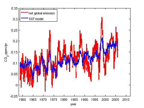
Figure 2: Regression model of net global emission as a function of sea surface temperature.
We can then compute the cumulatve sum to determine the effect of SSTs on the rise in atmospheric CO2 since 1959 (Figure 3).
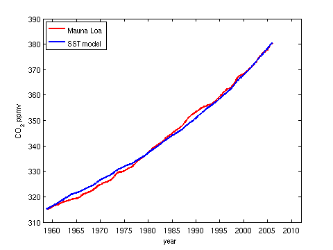
Figure 3: Modelled and observed increase in atmospheric CO2.
and it looks like it does a pretty good job. Unfortunately there are a couple of serious flaws in this line of reasoning. Firstly, if we look at the regression equation
NGE = 0.1688*SST + 0.1079
The additive constant at the end is a component of net global emission that cannot be explained by SSTs so we ought to delete it before we evaluate the cumulative sum, giving us this result:
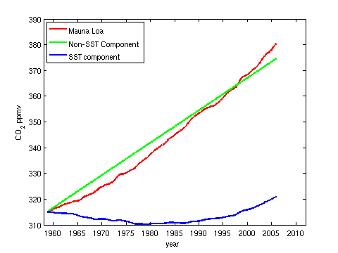
Figure 4: Decomposition of the modelled rise into components that are and are not explainable by SSTs.
Not quite so impressive!
The second problem with the regression analysis is an example of omitted variable bias; clearly anthropogenic emissions should be expected to have an effect on net global emission (all things being equal), and this was not included as an independent variable in the regression analysis. The physics of climate also tells us that surface temperatures (including SSTs) should also be increasing due to global warming. This means that SSTs are correlated with anthropogenic emissions. As regression is a correlation based technique this means that SSTs may explain net global emissions either because SSTs actually do affect net global emission, or because they act as a proxy for anthropogenic emissions, or both, and a simply regression analysis cannot tell which of these is actually correct. As a result, we cannot actually assert that the component due to SST actually represents a causal relationship between SSTs and net global emission.
Fortunately Dr Spencer includes anthropogenic emissions in his simple model of the carbon cycle,
?[CO2]/?[t] = a*SST + b*Anthro
where a and b are the coefficients, which in Dr Spencer's analysis are determined by manual experimentation, rather than by formal regression methods. Here, we will use a regression based approach, which has the advantage of being objective, giving the results shown in Figure 5.
Figure 5: Regression analysis based on the simple model proposed by Prof. Spencer
These results are not that similar to those of Spencer, but here they are at least optimal in a least-square sense, rather than being manually chosen. As SSTs and anthropogenic emissions are correlated, it is possible to construct a variety of models that explain the observations almost equally well, so manual search is vulnerable to unintended subjective bias. We will use the regresion based approach, but use an offset term as well, i.e.
?[CO2]/?[t] = a*SST + b*Anthro + c
as this gives better performance, shown in Figure 6.
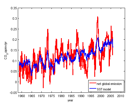
Figure 6: Model of net global emission based on SST and anthropogenic emissions.
Again, we can plot the contribution from each part of the model to the explanation of the increase in atmospheric CO2, giving:
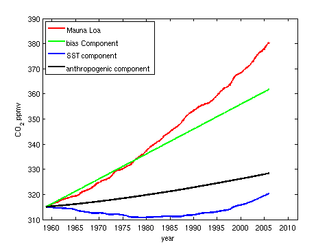
Figure 7: Attribution of the increase in atmospheric CO2 according to the regression model.
However, this model is still flawed, again due to omitted variable bias. While it is certainly true that the solubility of CO2 in the oceans decreases with increasing temperature, Henry's law tells us that the solubilty of CO2 also increases with an increasing difference in the partial pressures of CO2 in the atmosphere and in the surface waters. Thus as atmospheric CO2 increases, the net oceanic sink should increase, taking in more CO2. Thus atmospheric CO2 itself ought to be a variable included in the model. However, there is no real point in performing a yet more complex regression model. We already know the net anthropogenic and natural contribution to the observed increase, with high certainty, via the mass balance analysis.
Figure 8 shows a more realistic (subjective) attribution of the observed increase in atmospheric CO2. We know from the mass balance analysis that the annual rise is about twice the annual increase in atmospheric CO2, so in reality approximately 200% of the rise is anthropogenic. However, the natural environment is known to be a net sink, again via the mass balance analysis, and has been taking up about half of anthropogenic emissions each year. Thus the natural contribution to the observed increase is about -100%. Changes in SSTs do affect the annual growth rate of atmospheric CO2, but its effect is cyclical, so overall it does not lead to a significant long term trend in atmospheric CO2 (as discussed in the previous post), but just modulates atmospheric CO2 up and down slightly.
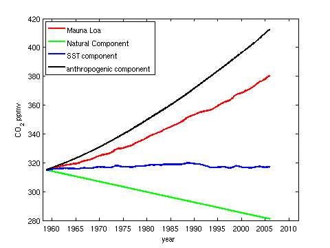
Figure 8: A more realistic attribution of the observed increase in atmospheric CO2
Key point: Trying to make causal arguments based on regression analysis is risky, especially if the underlying assumptions of regression analysis are violated, for instance because a relevant variable is omitted. Regression analysis is often used to show how much of Y can be explained by X. It is vital to remember that this does not imply that any of Y actually is explained by X. To make that leap, a plausible physical explanation is required that both explains the correlation and can also explain the magnitude of the observed effect. This is why we need to keep in mind that "correlation is not causation". Interesting correlations are a good stimulus to research, but at the end of the day we need the physics to support a causal link.
Posted by Dikran Marsupial on Saturday, 7 July, 2012
 |
The Skeptical Science website by Skeptical Science is licensed under a Creative Commons Attribution 3.0 Unported License. |