Because exponential growth of CO2 concentration causes only linear raise in temperature, people sometimes think that subsequent emissions will result in ever slower temperature increases. Well, the most persistent myths are based on technically true statements - that’s true also in this case.
It is true, that for each doubling of CO2 concentration, temperature increases by a constant value. However, at the current level of CO2 content in the atmosphere a good approximate relation is that for each 500 GtC (1833 bn tons of CO2) we can expect equilibrium temperature increase by approximately 1°C. Moreover, because of the continuing exponential growth of CO2 emissions the temperature increase will also accelerate.
When we talk about the temperature increase in response to the growth of greenhouse gases concentration in the atmosphere, we mean the total increase in average temperature which will continue until the Earth’s total energy budget reaches equilibrium. Both numerical simulations using climate models, as well as paleoclimatic research and direct measurements show that in response to doubling of the atmospheric CO2 concentration, (which is equivalent to a radiative forcing of 4W/m2), the Earth’s surface will most probably warm up by about 3°C.
Hence, we can expect a 3°C average temperature increase when the carbon dioxide concentration changes from the pre-industrial level of 280 ppm to 560 ppm. Subsequent temperature increase by another 3°C will require growth of CO2 concentration from 560 to 1120 ppm.
Should we therefore draw a conclusion that the rate of temperature increase will steadily drop? Not necessarily, and definitely not if current emissions trends persist in the future. In order to understand key relationships let’s take a look at the connection between our cumulative emissions and the projected temperature increase published in the 5th IPCC report.

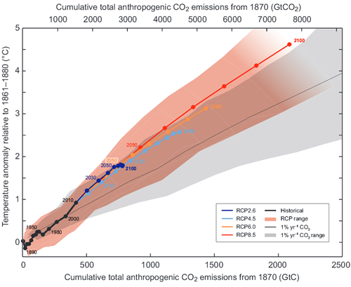
Figure 1: Increase of the mean Earth’s surface temperature as a function of the cumulative global CO2 emissions. Mean values calculated from multiple simulations using several carbon cycle models are shown until year 2100 for each RCP (color lines). Circles mark decadal means and for clarity selected decadal means were labeled with appropriate color matching text (e.g., 2050 indicates the decade 2040-2049). Black line denotes model results over the historical period (1860-2010). Shaded areas illustrate range of model results for various RCP scenarios. Black narrow line and grey shaded area show, respectively, the mean and the range of simulation results using many models CMIP5 assuming CO2 concentration growth of 1% per year. For a given value of cumulative CO2 emissions, simulations assuming 1% yearly concentration growth show smaller temperature increase than simulations corresponding to RCP, which include other forcings besides CO2. Temperature change is relative to the base period 1861-1881. Decadal averages are connected by straight lines. Source: 5th IPCC report.
The graph shows that the temperature increases almost linearly with the growth of cumulative emissions, and in case of “business as usual” scenario (red line RCP8.5) the temperature increase actually accelerates from decade to decade (as seen from the growing distance between circles marking subsequent decades). How can this observation be consistent with the logarithmic dependence between temperature increase and atmospheric CO2 concentration?
Let’s summarize several basic facts, which we will then use to reproduce Figure 1:
Table 1 contains results of simple calculations based on observations listed above. For example, if we assume that from the beginning of the industrial era the cumulative emissions were 500 GtC (equivalent to 1833 bn tons CO2), then the atmosphere absorbed 45% of the emitted CO2, or 225 GtC. As a result atmospheric CO2 concentration has increased by 225/2.12=106 ppm, reaching level of 386 ppm, which, in turn, increases the radiative forcing by 5.35·ln (386/280) = 1.72 [W/m2]. The expected (equilibrium) temperature rise will therefore be 3·1.72/3.7=1.39 [°C].
|
Cumulative emissions |
Left in the atmosphere [GtC] |
CO2 concentration [ppm] |
Radiative forcing RF |
Equilibrium |
| 0 | 0 | 280 | 0.00 | 0.00 |
| 500 | 225 | 386 | 1.72 | 1.39 |
| 1000 | 450 | 492 | 3.02 | 2.44 |
| 1500 | 675 | 598 | 4.06 | 3.29 |
| 2000 | 900 | 705 | 4.94 | 3.99 |
| 2500 | 1125 | 811 | 5.69 | 4.60 |
Table 1. Relationship between cumulative emissions and temperature anomaly. NOTE: our model (and Figure 1) considers only carbon dioxide emissions and does not include the effects of other greenhouse gases or the cooling effect of sulfuric aerosols (these two contributions are approximately cancelling each other).
The accuracy of our model is quite good (blue line in Figure 2).
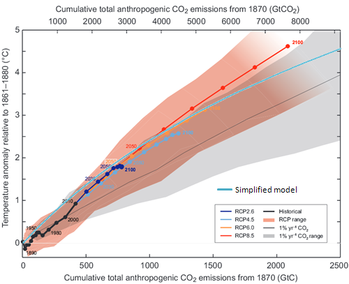
Figure 2. Results of our simple model calculations (light blue line) were added to data from Figure 1. MS Excel is available here.
Of course, such a model is very simplified. It assumes a constant airborne fraction (45%) of CO2 staying in the atmosphere. If emissions grew very fast, land and oceans sinks would be overwhelmed and would not keep pace absorbing our emissions, effectively causing larger portion of CO2 remaining in the atmosphere. According to Jones et. al., 2013, airborne fraction in RCP8.5 scenario for years 2006-2100 will go up to 69% (though uncertainity is quite large). Rising airborne fraction for huge emissions will straighten the curve. We also used the equilibrium temperature, while the real one will be somewhat smaller due to thermal inertia of the climate system.
If we include this in our model, assuming airborne fraction rising linearly from 45% (for 500 GtC of cumulative emissions) to 66% (for 2000 GtC) and display temperature anomaly as 80% of equilibrium temperature, we will get this:
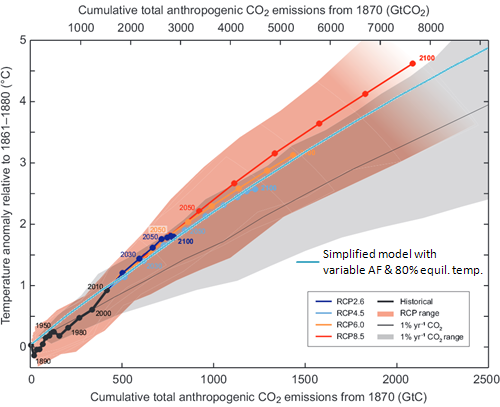
Figure 3. Results of our simple model calculations (light blue line) with variable airborne fraction and observed temperature as 80% of equilibrium temperature were added to data from Figure 1. MS Excel is available here.
We have reasonably well reproduced approximately linear relationship between cumulative emissions and the temperature anomaly, equivalent to about 1°C increase for each 500 GtC of emissions.
Exactly how quickly the temperature will rise will depend on the actual emissions rate.
Historical carbon dioxide emissions can be approximated using exponential function, i.e. one that grows by a constant factor every year. That means continually increasing growth rate. In Figure 4 an exponential function growing at a rate of 2.8% yearly was superimposed on the graph of historical CO2 emissions.
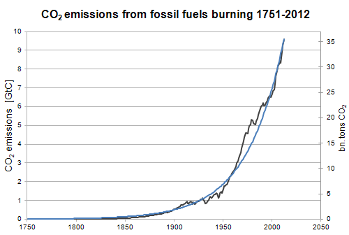
Figure 4. Growth of carbon dioxide emissions from burning fossil fuels during the period 1751-2012 (black line); source: CDIAC. Blue line represents exponential function growing at a rate of 2.8% per year (i.e. doubling every 25 years).
Such rate of growth means doubling the amount of CO2 emissions every 25 years. After 50, 75 and 100 years emissions become respectively 4 times, 8 times and 16 times larger. During the last 25 years we have emitted as much carbon dioxide from fossil fuels burning as from the beginning of the industrial revolution to the 1980s. More precisely, during 27 years between 1986 and 2012 we have emitted more CO2 than from 1751 to 1985 (CDIAC). Continuation of this trend would mean that between year 2010 and 2050 emissions would triple to a level of 100 bn tons of CO2 per year.
If the rate of emissions growth continues unchanged, in each subsequent decade we will dispose into the atmosphere ever increasing amounts of carbon dioxide, moving us ever faster to the right and upwards on the graph in Figure 1.
If we insist on burning everything we can, we will fulfill the RCP8.5 emissions scenario (or more).
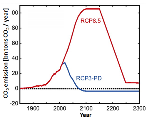
Figure 5. CO2 emissions according to two scenarios – burning all available fossil fuels (RCP 8.5) and one aiming at limiting temperature anomaly to below 2°C (RSP3-PD). In the extremely optimistic scenario RCP3-PD emissions are quickly reduced and in the middle of the XXI century fall below zero, which would mean enormous societal effort (during the lifetime of our children) of sequestration and removal from the carbon cycle of the CO2 emitted by our generation. Meinshausen et.al., 2011.
Emissions level as large as in the RCP8.5 scenario will introduce enough carbon into the carbon cycle to increase the Earth’s temperature by year 2100 by more than 4°C from the pre-industrial level (we can readily conclude this from Figure 1). Of course the temperature rise will not stop on 31 December 2100. If we assume that RCP8.5 emissions scenario continues into the next century, both axes of Figure 1 would have to be doubled in length. Simulations for this scenario (Meinshausen et.al., 2011) predict temperature anomaly by year 2200 of almost 8°C.
If we don’t change anything in our economic model (i.e. we will continue the ‘business-as-usual’ scenario), we may expect exponential growth of emissions and accelerated warming rate – in spite of “merely logarithmic” (as ‘skeptics’ emphasize) relationship between the CO2 concentration and the temperature anomaly.
Looking at Figure 1 we can immediately conclude, that if we seriously want to limit temperature anomaly to less than 2°C, we must keep the cumulative emissions below 1,000 GtC (3,666 bn tons CO2).
Marcin Popkiewicz, NaukaoKlimacie.pl; translation: Irek Zawadzki
Posted by Marcin Popkiewicz on Tuesday, 15 April, 2014
 |
The Skeptical Science website by Skeptical Science is licensed under a Creative Commons Attribution 3.0 Unported License. |