Illustrating periodic, apparent GW pauses.
We previously described events that cause energy to cycle between the oceans and the atmosphere at time scales on the order of years, to decades, and longer. To illustrate how the energy SeaSaw creates periodic, apparent pauses in global warming (GW), we combine two simple functions to show how they predict short-term, atmospheric cooling trends that are not indicative of long-term, GW trends.
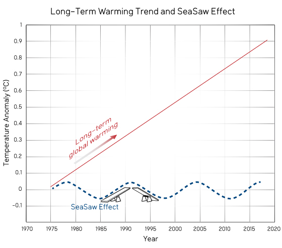
A sine wave describes the motion of many waves, such as those moving across a body of water. Imagine you are sitting stationary in a rubber boat on the ocean. The waves pass under you causing you to rise and fall in a pattern called “sinusoidal”. This is the approximate motion that represents the up-down pattern when two people use a teeter-totter.
The elevator motion is represented by an upward angled line, which shows the vertical position at a given time. If the elevator is rising with a constant speed of 1 m/s, then after 1 sec it will be 1 m above the ground, after 2 sec it will be 2 m above the ground, etc. Plotting the vertical position of the elevator (which can also be interpreted as the temperature anomaly) on one axis and time (i.e., current year) on the other axis produces an upward, slanted line. Figure 1 shows what the individual sinusoidal (SeaSaw) and constant-vertical motion (Elevator) traces look like, plotted as vertical position (temperature anomaly) vs. time (year).
Figure 1. Sinusoidal function (dotted line) plotted together with a constantly increasing function (solid line).
If we superimpose the SeaSaw and Elevator motions, the combined motion varies up and down relative to the Elevator-only line. This produces the motion shown in Fig. 2.
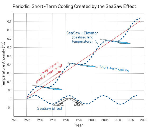
Figure 2. Idealized atmospheric temperature obtained by combining the sinusoidal and constant function shown in Fig. 1 to illustrate the oscillating, upward trend. Notice the short-term, periodic cooling followed by rapid temperature increase.
Figure 2 shows an interesting effect. Even though the elevator is going up, during some short-term intervals the vertical position of one end of the seesaw goes down, not up! This is comparable to short-term trends when atmospheric temperatures decrease, even though the long-term trend clearly shows warming. However, these short-term cooling trends are followed by rapid warming, so that the overall motion over a sufficiently long time is given by the long-term, upward trend.
As you might expect, we cannot hope to model atmospheric temperatures using a single sinusoidal function combined with a single upward trend. Earth’s land-ocean interactions are far more complicated, and include many variations with intervals both shorter and longer periods than shown in Figs. 1 and 2. However, just to see how close we come to approximating the varying global warming signal by using a single, simple sinusoidal function, Fig. 3 shows measured land temperatures superimposed on top of the combined SeaSaw signal. The comparison shown in Fig. 3 indicates that a single sinusoidal function combined with a single upward trend does a very good job of explaining the temporary up’s and down’s of the measured land temperatures.
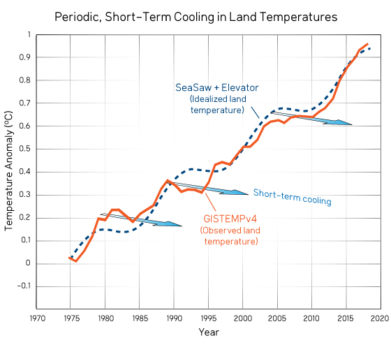
Figure 3. Observed land temperatures (GISTEMPv4) superimposed on top of the idealized land temperature from Fig 2.
Posted by Evan on Thursday, 27 May, 2021
 |
The Skeptical Science website by Skeptical Science is licensed under a Creative Commons Attribution 3.0 Unported License. |