There is much discussion about reducing our carbon footprint to stabilize climate. Many companies pledging to become carbon neutral, some pledging to remove all of their legacy carbon emissions, one car company after another announcing new lines of sleek EV’s. We will need all of these efforts, and more, because as of 2020, the IPCC consensus is that to avoid the worst effects of GW/CC, we must achieve the following, twin objectives:
Becoming carbon neutral is needed to stop GHGs from continuing to build up in the atmosphere and hopefully decrease atmospheric CO2 concentrations. Staying well below 2°C is needed to limit climate change to a level to which human civilization can adapt.
Are these twin goals realistic? What will it take to achieve them? If the best we can do is to achieve Net-0 Accumulation, but not necessarily by 2050, to what level of warming will we stabilize climate? Regardless of our best intentions, there may be limits on how much we can do and how fast. Like a super-tanker plying the oceans at top speed, there are physical limits on how fast course corrections can be made. Sociological limits determine how fast we can mobilize effective action. As of 2021, none of the talk, high-level negotiations, nor even a pandemic has altered the persistent, upward trajectory of CO2 as represented by the Keeling Curve.
There are also technical and monetary issues. We know how to decarbonize the energy sector using wind, solar, battery storage, EV’s, and other current and up-and-coming technologies such as nuclear, and hopefully someday, fusion power. It will take time, but we are well on our way to doing it and low-carbon energy is already cheaper than building new fossil-fuel power plants. Decarbonizing the energy sector, however, is not sufficient to stabilize climate. We must also remove CO2 from the atmosphere to balance GHG emissions from sectors that are difficult to decarbonize, such as agriculture. Although land-use modifications are being studied as ways to increase the CO2 uptake by the biosphere, drawing down CO2 concentrations at a rate required to stabilize CO2 concentrations will likely require artificial, mechanical means as well.
Because agricultural, baseline emissions cannot be easily eliminated, they must be compensated for by using Negative Emissions Technologies (NET) to extract an equal amount of GHGs directly from the air. Estimates by Larkin et al. (2014) suggest that baseline emissions amount to about 1 ton CO2e/person/yr.1 We use this average value from Larken et al. to approximate how the baseline emissions scale with population, and the implications for the level of NET required to offset them. For the purposes of the modeling scenarios described here, we treat the non-CO2 baseline emissions as all CO2. We refer to the CO2 accumulation due to baseline emissions as Baseline Accumulation Rates (BAR).
There are three challenges to deploying NET systems at a scale sufficient to counteract human GHG emissions.
It may be that the issue of delayed benefit is more difficult to sell to the public than the cost of implementing carbon-neutral solutions.
NET systems refer to a suite of remedies, from enhancing natural carbon uptake of the biosphere by modified farming practices and reforestation, to brute-force, direct-air capture of CO2 and burying it in suitable underground storage sites. Also, some NET systems may compete with each other for available land area. Deforestation is occurring largely because of the desire to increase available agricultural land area. This trend must be opposed at the same time that we seek to increase the land area used for NET systems. As of 2021, NET systems are at various stages of development. It is uncertain if any are ready for wide-scale deployment, because this requires not only technical capabilities, but the logistics of deploying a system that will rival the scale of international shipping and commerce.
This article lays out some optional paths we can choose and the destinations to which they take us. Some GHG-mitigation paths will be harder to follow than others, and will require concerted international will and lots of creative science and engineering, some yet to be developed. We use a simple model to illustrate some of the potential scenarios for stabilizing atmosphere CO2 concentrations. Details of this model are given in the Appendix.
The purpose of this model is not so much to make specific predictions, but rather to 1) illustrate the challenges of stabilizing climate, and to 2) define methods for monitoring our progress towards the IPCC goals. The IPCC has been issuing various levels of warnings since 1990, which society has been slow to heed. My goal is to help you assess our progress towards meeting the IPCC goal of stabilizing atmospheric temperatures to well below 2°C.
There are four processes that determine atmospheric CO2 concentrations
By definition, atmospheric CO2 concentrations stabilize when the sources are balanced by the sinks, and atmospheric CO2 concentrations decrease when the sinks exceed the sources. The Keeling Curve tells us the state of the balance or imbalance of these four processes, because the Keeling Curve represents the CO2 accumulated in the atmosphere due to the net effect of these four processes. The best way to monitor our progress towards the IPCC goals is, therefore, to monitor the progress of the Keeling Curve.
The current upward acceleration of the Keeling Curve indicates that as of 2021, the sources far exceed the sinks. The first goal, therefore, is to achieve Net-0 Accumulation: to balance the sources with the sinks. As long as we can maintain Net-0 Accumulation, we will cap the warming. That alone will be a huge achievement!
But achieving the first goal is not enough. The second goal is to increase the sinks, so that they exceed the sources, bringing down CO2 concentrations and capping the warming at a level that is lower than is possible with Net-0 Accumulation alone. This second goal is needed to not just cap the warming, but to cap it at a level that improves the odds that humans successfully adapt to the new climate.
The path to becoming carbon neutral is by 1) transitioning energy systems completely away from fossil fuels and replacing them with low-carbon energy sources, which we refer to as an Energy Transition, and by 2) deploying NET systems at a scale sufficient to achieve Net-0 Accumulation. I approximate this NET level by equating it to the Baseline Accumulation Rate (BAR). Deploying NET at a rate larger than BAR is needed to deal with legacy emissions: we must also suck sufficient CO2 out of the air to reduce the CO2 concentration to a level that corresponds to a temperature anomaly well below 2°C. Whether or not you accept the level of baseline emissions described by Larkin et. al. (2014), the important point is that there is one level of NET that will be needed to cap the warming. But because that level of stabilization will likely exceed 2°C, we will have to continue to deploy NET until we stabilize temperature well below 2°C. The reason for showing simulations at two different levels of NET, therefore, is to emphasize this 2-step path to meeting the IPCC twin goals.
The Paris Accord states that to avoid the worst effects of global warming, that we must maintain temperature anomalies well below 2°C. This corresponds to a CO2 concentration less than 450 ppm. As of 2020, CO2 concentrations are above 410 ppm, enough to raise temperatures to about 1.6°C. Because of a 30-year delay between achieving a given CO2 concentration and the temperature increase associated with that CO2 level, as of 2020 the temperature anomaly is still only about 1.1°C. While temperatures are increasing, the thermal inertia of the Earth helps us by delaying the warming associated with a given CO2 concentration. This gives us time to reduce CO2 levels before the temperature catches up. However, should we allow the temperature to increase to 2°C or above, and then use NET systems to reduce atmospheric CO2 concentration, the thermal inertia will work against us, stubbornly keeping temperatures higher than associated CO2 concentrations would dictate. Elevated temperatures increase the risk of activating feedback processes, so that in addition to thermal inertia working against us, excursions above 2°C bring other risks for triggering feedback processes. Therefore, even a “temporary” temperature excursion above the IPCC 2°C limit increases risks substantially.
Professional climate modelers start with GHG emission rates and model the fate of those GHG emissions once they enter the atmosphere: ultimately, they are either absorbed by the biosphere or accumulate in the atmosphere. Future, hypothetical emission scenarios together with assumptions about the evolution of the biosphere CO2 uptake are proposed to see how they impact atmospheric accumulation rates. Such models require detailed emission-rate scenarios and estimates of the rates of uptake by different parts of the biosphere. But one of the ultimate goals of climate models is to simulate the evolution of atmospheric GHG accumulation rates, specifically, atmospheric CO2 accumulation rates.
Rather than simulate the detailed fate of GHG emissions, I formulated a simpler model that directly simulates societal factors on atmospheric CO2 accumulation. As such, I formulated the model directly in terms of measured CO2 accumulation rates in the atmosphere, and I directly relate those CO2 accumulation rates to population, affluence, and the carbon footprint of producing goods and services. From historical records, we know how rapidly population, affluence, and the carbon intensity of industry has been changing and we can relate them to known changes in atmospheric CO2 accumulation rates. By making estimates of how population, affluence, and industrial carbon intensity are likely to change in the future, we can use this simple model to estimate how future CO2 accumulation rates are likely to change.
The model I used is a form of the so-called IPAT equation (i.e., I = P × A × T), The Appendix shows details of the model results presented here, which relates the Impact (I) on the environment due to Population (P), Affluence (A), and Technology (T). In my model, Impact is defined as atmospheric CO2 accumulation, Affluence is measured in World GDP (WGDP) per person, and Technology is measured in CO2 accumulation in the atmosphere per unit WGDP required to produce our goods and services.
As of 2020, global population is increasing by 80,000,000 people per year, WGDP/person is increasing about 2%/year, and the carbon footprint per unit WGDP of producing goods and services is decreasing about 2%/year, offsetting rising consumption. Because CO2 has been rapidly increasing during a period of steady reductions in CO2 emissions per unit WGDP, to stabilize atmospheric CO2 we will have to do much better than a decrease of 2%/year.
A credible population model (read here and here) suggests that global population growth could be slowing sufficiently so that it peaks and stabilizes by mid-century at 9 billion. We assume this population model to be correct. We further assume that current consumption patterns continue unchanged. This means that from 2020 to 2100 that the average per-capita consumption continues to increase at the same rate as from 1990 to 2020, at about 2%/person/yr. There is nothing in our experience to suggest that the world, as a whole, will accept stagnating standards of living. Developed countries want to consume more, developing countries want to raise their populations out of poverty. People may accept taxes required to stabilize the climate, but it is unlikely they will accept forced austerity measures for an extended period of time.
Current models suggest that once we achieve Net-0 Emissions, that natural biosphere carbon sinks will slowly draw down CO2. The net effect is that temperatures will stabilize at that point and remain at that level for multiple centuries (Hausfather, 2021, and Matthews and Caldiera, 2008). We therefore assume that once CO2 begins to drop, that temperatures stabilize at that level.
Conceptually, if we transition away from burning fossil fuels to producing electricity by using low-carbon energy, we can reduce the carbon footprint of non-agricultural consumables. For the transition from fossil fuels to renewable energy, we model the following scenarios:
For agricultural emissions and other sectors for which it is difficult to eliminate all GHG emissions, BAR is determined by the population: more people means more food produced and consumed. Because BAR must be compensated using NET, there are two levels of NET modeled
NOTE: Some will argue, based on the work of Matthews and Caldiera (2008), that if we negate baseline emissions, by equating NET to BAR, that this should be sufficient to cause atmospheric CO2 to decrease, instead of just stabilizing atmospheric CO2 concentration, as assumed in this model. However, the numbers and assumptions used in this model are illustrative, and should not be interpreted as quantitative estimates of future emissions. As Hausfather (2021) noted,
Even in a world of zero CO2 emissions, however, there are large remaining uncertainties associated with what happens to non-CO2 greenhouse gases (GHGs), such as methane and nitrous oxide, emissions of sulphate aerosols that cool the planet and longer-term feedback processes and natural variability in the climate system.
We therefore do not assume that equating NET to BAR will be sufficient to stabilize temperature. However, the main points that we are trying to emphasize with this model are
Therefore, I assume that equating NET to BAR is sufficient to stabilize CO2 concentrations. What’s actually needed might be more or less than this level, but equating NET to BAR is a good rough estimate of the level that will likely be needed.
The assumptions of population stabilizing by mid-century at 9 billion people and global consumption increasing 2%/yr are common to all of the following scenarios. The differences in the following scenarios are the rate of the Energy Transition associated with decarbonizing as much of society as possible, and the magnitude of NET. I show the results of four scenarios, summarized in Table 1.
Table 1. Modeling scenarios included in this chapter. All scenarios assume that population growth stabilizes by mid-century at 9 billion people.
| Scenario | Consumption | Decarb. Rate | NET |
| Business as Usual (BAU) | +2%/yr | -2%/yr | none |
| Energy Transition | +2%/yr | -4%/yra | none |
| Accelerated Energy Transition + NET | +2%/yr | -8%/yrb | =BARc |
| Accelerated Energy Transition + 2NET | +2%/yr | -8%/yr | =2BARd |
a. 10-year transition from base rate of -2%/yr up to -4%/yr
b. 10-year transition from base rate of -2%/yr up to -8%/yr
c. Beginning deployment in 2030 and requiring 20 years for full deployment.
d. Beginning deployment in 2030 and requiring 30 years for full deployment.
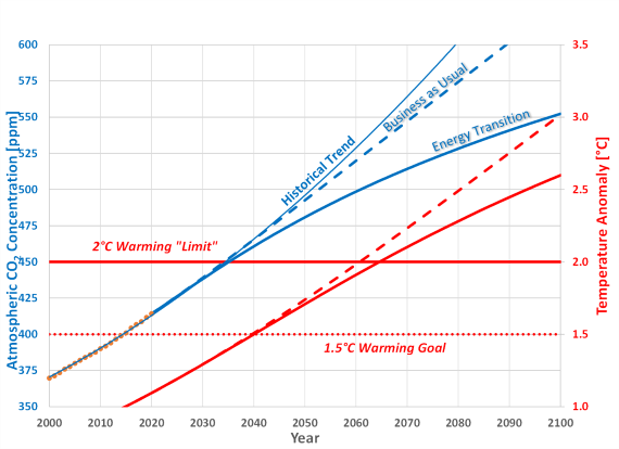
Figure 1 shows atmospheric CO2 concentration and temperature trends for the BAU and Energy Transition scenarios defined in Table 1. The left, vertical axis shows the CO2 concentration, and the right, vertical axis shows the corresponding temperature anomaly. For example, the dashed, blue line shows the atmospheric CO2 concentration on the left, vertical axis, and the dashed, red line shows the warming to which that level of CO2 corresponds, on the right, vertical axis. The temperature trends include the effects of a 30-year delay between atmospheric CO2 accumulation and when the temperature catches up.
Figure 1. Atmospheric CO2 concentration up to 2100 for the BAU and Energy Transition scenarios. The left, vertical axis shows the CO2 concentration, and the right, vertical axis shows the corresponding temperature anomaly.
Figure 1 indicates that the BAU scenario blows past 2°C warming by 2060 and does not lead to climate stabilization. The Energy Transition scenario does marginally better, but still breaches 2°C warming by 2065, and also does not lead to climate stabilization. That is, simply transitioning from burning fossil fuels to using low-carbon energy is not sufficient to stabilize climate.
Figure 2 shows atmospheric CO2 concentration and temperature trends for the remaining two scenarios. Adding NET is sufficient to stabilize CO2 concentrations, but even with the Accelerated Energy Transition and under the ideal conditions of this model, stabilization occurs in excess of 2°C warming. Stabilizing temperature below 2°C requires deploying NET at twice BAR.
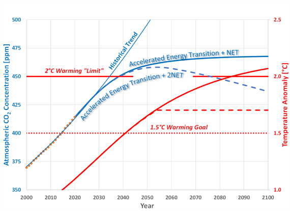
Figure 2. Atmospheric CO2 concentration up to 2100 for the Accelerated Energy Transition scenarios. The left, vertical axis shows the CO2 concentration, and the right, vertical axis shows the corresponding temperature anomaly.
Note that in the Accelerated Energy Transition + 2NET scenario, that shortly after 2050 CO2 begins to fall. According to Matthew and Caldiera (2008), when this happens, temperatures should stabilize. The key point is that deploying NET at a level sufficient to get atmospheric CO2 to start decreasing is needed to stabilize temperatures below 2°C.
KEY POINT: When the IPCC issued their first report in 1990, to stabilize temperatures below 2°C it was sufficient to stabilize CO2 concentrations. That is, achieving Net-0 Accumulation would have been sufficient to stabilize temperature below 2°C. In 2021 stabilizing CO2 concentration is no longer sufficient to keep temperature anomalies below 2°C: we must now go beyond stabilization of CO2 concentrations and bring them down.
When we see the problem in the perspective presented here, with everything clearly laid out, we like to believe that we will respond aggressively and responsibly. But a large part of the world either does not view the problem as presented here, or they have other priorities that prevent them from committing to the action needed. One challenge will be to maintain the needed focus for the better part of a century. This analysis shows that the sooner we tackle the energy transition, the easier it will be to achieve the emissions goals laid out by the Paris Accord.
The purpose of this simple model is to illustrate the challenges for stabilizing the climate. This is not a prediction of what will happen, just an illustration of what it will take to do what we need to do. Hopefully this helps you understand the extreme measures that governments may be proposing in the coming years. Although there is much talk about removing CO2 from the atmosphere, nature took 10’s of millions of years to bury it in the ground, and the easiest way to stabilize atmospheric CO2 concentrations is to take advantage of what nature did for us by burying it, and to leave as much in the ground as we can. It is beneficial to understand the magnitude of the problem so that this knowledge can motivate us to move as fast as possible towards a more sustainable lifestyle.
Talk to others and share this information. Talking to others about these issues is one of the most important things you can do to help stabilize the climate.
Hausfather, Z (2021), Will global warming ‘stop’ as soon as net-zero emissions are reached?, Carbon Brief.
Larkin, A.B., Carly McLachlan, Sarah Mander, Ruth Wood, Mirjam Röder, Patricia Thornley, Elena Dawkins, Clair Gough, Laura O’Keefe & Maria Sharmina (2014) Importance of non-CO2 emissions in carbon management, Carbon Management, 5:2, 193-210.
Matthews, H.D. and Caldiera, K (2008), Stabilizing climate requires near-zero emissions, Geophysical Research Letters.
The factors driving up annual CO2 accumulation rates are (1) the number of people, represented by the global population, (2) total consumption, expressed as WGDP, and (3) the carbon footprint of producing our goods and services, expressed as the CO2 accumulation in the atmosphere per unit WGDP.
We develop a model directly in terms of the accumulation of CO2 in the atmosphere, and not CO2 emissions, because it is the accumulation of CO2 in the atmosphere that controls climate. The relationship between the two is that as of 2020 about half of our CO2 emissions remain in the atmosphere and the other half are absorbed by the biosphere.
A relationship for CO2 accumulating in the atmosphere and sociological factors, based on the so-called IPAT equation, can be written as
![]()
The first term represents the Baseline Accumulation Rate (BAR) that must be counteracted using Negative Emissions Technology (NET), whereas the second term represents the effect of processes to produce our goods and services, which we assume can be virtually eliminated by shifting from an economy based on fossil-fuel combustion to one based on low-carbon energy. The goal is to eliminate the effect of the second term through an Energy Transition from burning fossil fuels to using low-carbon energy.
I used information about historical trends to estimate how rapidly we might be able to ramp down atmospheric CO2 accumulation. With an estimate for (Baseline CO2)/Person of about 1 ton-CO2e/yr/person, we can estimate both historical and future BAR simply by knowing the global population. To estimate the contribution of the energy term, we note that atmospheric CO2 concentrations are measured daily, and therefore ΔCO2/yr is known for past years. We also have estimates of past population and WGDP. Although ΔCO2/WGDP is not a quantity that we can easily measure, from the other, known terms in this relationship, we can calculate historical values of ΔCO2/WGDP. Calculated values indicate that ΔCO2/WGDP has been decreasing since the mid 1970’s at a rate of about 2%/yr. Knowing the rate at which ΔCO2/WGDP has been decreasing in recent decades, we can estimate future rates of decrease by assuming they continue to decrease at similar or accelerated rates. For example, if we double our efforts to fight climate change, then in some sense we can expect ΔCO2/WGDP to decrease in the future at twice the historical rate.
This model directly represents the effect of the model parameters of population, consumption, and the carbon footprint of producing goods and services on the rate of accumulation of CO2 in the atmosphere. We use historical trends of the controlling parameters to project forward into the future, combined with estimates of the time required to execute transitions from fossil-fuel based energy production to low-carbon energy production. For example, even though in 2020 the transition to low-carbon energy is already underway, we assume that any attempt to accelerate the transition will take 10 years, reflecting estimates for the time for legislative action, the time to ramp up the requisite industry, and the time to accelerate installations. Should we succeed in affecting such transitions faster than 10 years, then 10 years simply represents a conservative estimate.
This model does not rely on knowing detailed emissions inventories of various sectors of society. The model parameters are based on extensions of past, overall trends into the future.
Table 2 shows historical values of the model parameters. Whereas historical CO2 concentrations and population data are readily available, WGDP is only available from 1990, because to be useful in this comparison as a global parameter, it must be adjusted for local Purchasing Power Parity (PPP) in all countries, and must also be inflation adjusted to a given year. The WGDP data set used in this analysis only goes back to 1990.
Table 2 indicates that in 1970 atmospheric CO2 increased about 1.1 ppm/yr. In 1970 the global population was about 3.7 billion and by 2015 it had doubled to about 7.4 billion. Over the same period, large improvements were made in the energy efficiency of cars, planes, home heating and insulation, as well as a general reduction of the carbon footprint of industrial processes. With this reduction of the carbon footprint of producing goods and services, one might expect that CO2 accumulation rates decreased. However, in 2015 CO2 increased by more than 2.3 ppm/year, indicating that in 2015 the per-capita CO2 accumulation in the atmosphere was nearly the same as in 1970. The decreasing carbon footprint of producing goods and services was offset by increasing per-capita consumption. If the average per-person production of CO2 was constant, that means that from 1970 to 2015 the rise in global population drove the acceleration of CO2 accumulation in the atmosphere. Because the per-capita consumption varies greatly from developed to developing countries, the situation is more complex that presented here, but the point of this analysis is to broadly define the effect of the three major drivers of CO2 accumulation: population, consumption, and the carbon footprint of converting WGDP into goods and services.
Table 2. Historical values of the model parameters: average annual changes of CO2, global population, and WGDP from 1970 to 2020. ΔCO2/WGDP is calculated from measured CO2 concentrations and WGDP.
|
Year |
CO2 [ppm] |
ΔCO2/yr [ppm]a |
Baseline ΔCO2b |
Energy ΔCO2c | Popd | WGDPe |
WGDP/ Personf |
ΔCO2/ WGDPg |
|---|---|---|---|---|---|---|---|---|
| 1970 | 326 | 1.10 | 0.25 | 0.85 | 3.70 | |||
| 1980 | 339 | 1.36 | 0.30 | 1.06 | 4.46 | |||
| 1990 | 355 | 1.61 | 0.36 | 1.25 | 5.33 | 51 | 9,600 | 2.58 |
| 2000 | 370 | 1.87 | 0.42 | 1.45 | 6.14 | 68 | 11,000 | 2.17 |
| 2010 | 391 | 2.13 | 0.48 | 1.65 | 6.96 | 96 | 13,800 | 1.77 |
| 2020 | 414 | 2.38 | 0.53 | 1.85 | 7.80 | 130 | 17,100 | 1.37 |
I assume that WGDP/Person continues to increase into the future at the same rate as from 1990 to 2020. I assume that population stabilizes by 2050 at 9 billion people. Although an optimistic scenario for population growth, it is one that is backed by a reputable study (read here and here). Because countries can encourage or discourage population growth, population may be a model factor that can, to some extent, be influenced. We therefore use this optimistic population model, because this model demonstrates the difficulty of meeting the Paris Accord goals, even with an optimistic population model. The Energy Transition scenarios are formed by assuming that the historical rate of ΔCO2/ WGDP increases by either a factor of 2 or 4. This, of course, depends on how aggressively countries push for the transition to low-carbon energy.
Posted by Evan on Tuesday, 9 November, 2021
 |
The Skeptical Science website by Skeptical Science is licensed under a Creative Commons Attribution 3.0 Unported License. |