This is part 2 of a guest post by KK Tung, who requested the opportunity to respond to the SkS post Tung and Zhou circularly blame ~40% of global warming on regional warming by Dumb Scientist (DS).
In this second post I will review the ideas on the Atlantic Multidecadal Oscillation (AMO). I will peripherally address some criticisms by Dumb Scientist (DS) on a recent paper (Tung and Zhou [2013] ). In my first post, I discussed the uncertainty regarding the net anthropogenic forcing due to anthropogenic aerosols, and why there is no obvious reason to expect the anthropogenic warming response to follow the rapidly increasing greenhouse gas concentration or heating, as DS seemed to suggest.
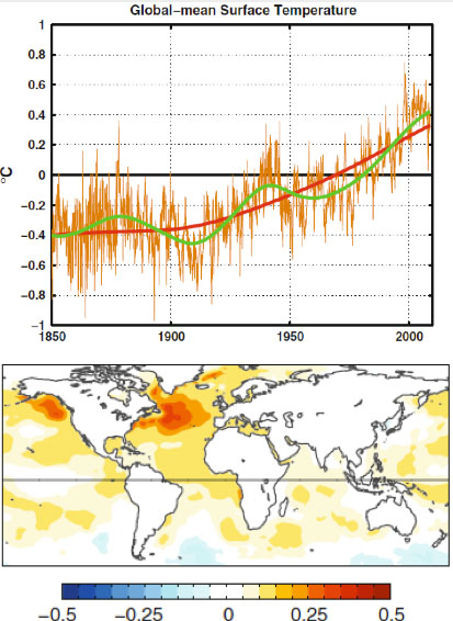
For over thirty years, researchers have noted a multidecadal variation in both the North Atlantic sea-surface temperature and the global mean temperature. The variation has the appearance of an oscillation with a period of 50-80 years, judging by the global temperature record available since 1850. This variation is on top of a steadily increasing temperature trend that most scientists would attribute to anthropogenic forcing by the increase in the greenhouse gases. This was pointed out by a number of scientists, notably by Wu et al. [2011] . They showed, using the novel method of Ensemble Empirical Mode Decomposition (Wu and Huang [2009 ]; Huang et al. [1998] ), that there exists, in the 150-year global mean surface temperature record, a multidecadal oscillation. With an estimated period of 65 years, 2.5 cycles of such an oscillation was found in that global record (Figure 1, top panel). They further argued that it is related to the Atlantic Multi-decadal Oscillation (AMO) (with spatial structure shown in Figure 1, bottom panel).
Figure 1. Taken from Wu et al. [2011] . Top panel: Raw global surface temperature in brown. The secular trend in red. The low-frequency portion of the data constructed using the secular trend plus the gravest multi-decadal variability, in green. Bottom panel: the global sea-surface temperature regressed onto the gravest multi-decadal mode.
Less certain is whether the multidecadal oscillation is also anthropogenically forced or is a part of natural oscillation that existed even before the current industrial period.
It is now known that the AMO exists in coupled atmosphere-ocean models without anthropogenic forcing (i.e. in “control runs”, in the jargon of the modeling community). It is found, for example in a version of the GFDL model at Princeton, and the Max Planck model in Germany. Both have the oscillation of the right period. In the models that participated in IPCC’s Fourth Assessment Report (AR4), no particular attempt was given to initialize the model’s oceans so that the modeled AMO would have the right phase with respect to the observed AMO. Some of the models furthermore have too short a period (~20-30 years) in their multidecadal variability for reasons that are not yet understood. So when different runs were averaged in an ensemble mean, the AMO-like internal variability is either removed or greatly reduced. In an innovative study, DelSol et al. [2011] extract the spatial pattern of the dominant internal variability mode in the AR4 models. That pattern (Figure 2, top panel) resembles the observed AMO, with warming centered in the North Atlantic but also spreading to the Pacific and generally over the Northern Hemisphere (Delworth and Mann [2000] ).
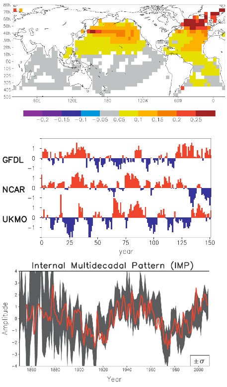
Figure 2. Taken from DelSol et al. [2011] . Top panel: the spatial pattern that maximizes the average predictability time of sea-surface temperature in 14 climate models run with fixed forcing (i.e. “control runs”). Middle panel: the time series of this component in three representative control runs. Bottom panel: time series obtained by projecting the observed data onto the model spatial pattern from the top panel. The red curve in the bottom panel is the annual average AMO index after scaling.
When the observed temperature is projected onto this model spatial pattern, the time series (in Figure 2 bottom panel) varies like the AMO Index (Enfield et al. [2001] ), even though individual models do not necessarily have an oscillation that behaves exactly like the AMO Index (Figure 2, middle panel).
There is currently an active debate among scientists on whether the observed AMO is anthropogenically forced. Supporting one side of the debate is the model, HadGEM-ES2, which managed to produce an AMO-like oscillation by forcing it with time-varying anthropogenic aerosols. The HadGEM-ES2 result is the subject of a recent paper by Booth et al. [2012] in Nature entitled “Aerosols implicated as a prime driver of twentieth-century North Atlantic climate variability”. The newly incorporated indirect aerosol effects from a time-varying aerosol forcing are apparently responsible for driving the multi-decadal variability in the model ensemble-mean global mean temperature variation. Chiang et al. [2013] pointed out that this model is an outlier among the CMIP5 models. Zhang et al. [2013] showed evidence that the indirect aerosol effects in HadGEM-ES2 have been overestimated. More importantly, while this model has succeeded in simulating the time behavior of the global-mean sea surface temperature variation in the 20th century, the patterns of temperature in the subsurface ocean and in other ocean basins are seen to be inconsistent with the observation. There is a very nice blog by Isaac Held of Princeton, one of the most respected climate scientists, on the AMO debate here. Held further pointed out the observed correlation between the North Atlantic subpolar temperature and salinity which was not simulated with the forced model: “The temperature-salinity correlations point towards there being a substantial internal component to the observations. These Atlantic temperature variations affect the evolution of Northern hemisphere and even global means (e.g., Zhang et al 2007). So there is danger in overfitting the latter with the forced signal only.”
The salinity-temperature co-variation that Isaac Held mentioned concerns a property of the Atlantic Meridional Overturning Circulation (AMOC) that is thought to be responsible for the AMO variation at the ocean surface. This Great Heat Conveyor Belt connects the North Atlantic and South Atlantic (and other ocean basins as well), and between the warm surface water and the cold deep water. The deep water upwells in the South Atlantic, probably due to the wind stress there (Wunsch [1998] ). The upwelled cold water is transported near the surface to the equator and then towards to the North Atlantic all the way to the Arctic Ocean, warmed along the way by the absorption of solar heating. Due to evaporation the warmed water from the tropics is high in salt content. (So at the subpolar latitudes of the North Atlantic, the salinity of the water could serve as a marker of where the water comes from, if the temperature AMO is due to the variations in the advective transport of the AMOC. This behavior is absent if the warm water is instead forced by a basin wide radiative heating in the North Atlantic.) The denser water sinks in the Arctic due to its high salt content. In addition, through its interaction with the cold atmosphere in the Arctic, it becomes colder, which is also denser. There are regions in the Arctic where this denser water sinks and becomes the source of the deep water, which then flows south. (Due to the bottom topography in the Pacific Arctic most of the deep water flows into the Atlantic.) The Sun is the source of energy that drives the heat conveyor belt. Most of the solar energy penetrates to the surface in the tropics, but due to the high water-vapor content in the tropical atmosphere it is opaque to the back radiation in the infrared. The heat cannot be radiated away to space locally and has to be transported to the high latitudes, where the water vapor content in the atmosphere is low and it is there that the transported heat is radiated to space.
In the North Atlantic Arctic, some of the energy from the conveyor belt is used to melt ice. In the warm phase of the AMO, more ice is melted. The fresh water from melting ice lowers the density of the sinking water slightly, and has a tendency to slow the AMOC slightly after a lag of a couple decades, due to the great inertia of that thermohaline circulation. A slower AMOC would mean less transport of the tropical warm water at the surface. This then leads to the cold phase of the AMO. A colder AMO would mean more ice formation in the Arctic and less fresh water. The denser water sinks more, and sows the seed for the next warm phase of the AMO. This picture is my simplified interpretation of the paper by Dima and Lohmann [2007] and others. The science is probably not yet settled. One can see that the physics is more complicated than the simple concept of conserved energy being moved around, alluded to by DS. The Sun is the driver for the AMOC thermohaline convection, and the AMO can be viewed as instability of the AMOC (limit cycle instability in the jargon of dynamical systems as applied to simple models of the AMOC).
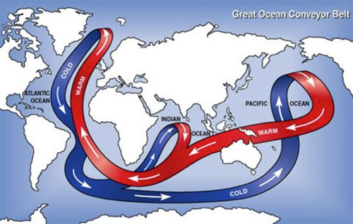
Figure 3. The great ocean conveyor belt. Schematic figure taken from Wikipedia.
It is fair to conclude that no CMIP3 or CMIP5 models have successfully simulated the observed multidecadal variability in the 20th century using forced response. While this fact by itself does not rule out the possibility of an AMO forced by anthropogenic forcing, it is not “unphysical” to examine the other possibility, that the AMO could be an internal variability of our climate system. Seeing it in models without anthropogenic forcing is one evidence. Seeing it in data before the industrial period is another important piece of evidence in support of it being a natural variability. These have been discussed in our PNAS paper. Figure 4 below is an updated version (to include the year 2012) of a figure in that paper. It shows this oscillation extending back as far as our instrumental and multi-proxy data can go, to 1659. Since this oscillation exists in the pre-industrial period, before anthropogenic forcing becomes important, it plausibly argues against it being anthropogenically forced.
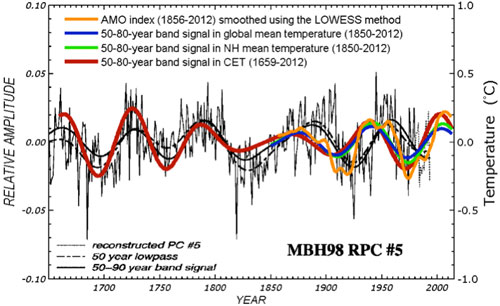
Figure 4. Comparison of the AMO mode in Central England Temperature (CET) (red) and in global mean (HadCRUT4) (blue), obtained from Wavelet analysis, with the multi-proxy AMO of Delworth and Mann [2000] (in thin black line). The amplitude of multi-proxy data is only relative (left axis). The orange curve is a smoothed version of the AMO index originally available in monthly form.
The uncertainties related to this result are many, and these were discussed in the paper but worth highlighting here. One, there is no global instrumental data before 1850. Coincidentally, 1850 is considered the beginning of the industrial period (the Second Industrial Revolution, when steam engines spewing out CO2 from coal burning were used). So pre-industrial data necessarily need to come from nontraditional sources, and they all have problems of one sort of the other. But they are all we have if we want to have a glimpse of climate variations before 1850. The thermometer record collected at Central England (CET) is the longest such record available. It cannot be much longer because sealed liquid thermometers were only invented a few years earlier. It is however a regional record and does not necessarily represent the mean temperature in the Northern Hemisphere. This is the same problem facing researchers who try to infer global climate variations using ice-core data in the Antarctica. The practice has been to divide the low-frequency portion of that polar data by a scaling factor, usually 2, and use that to represent the global climate. While there has been some research on why the low-frequency portion of the time series should represent a larger area mean, no definitive proof has been reached, and more research needs to be done. We know that if we look at the year-to-year variations in winters of England, one year could be cold due to a higher frequency of local blocking events, while the rest of Europe may not be similarly cold. However, if England is cold for 50 years, say, we know intuitively that it must have involved a larger scale cooling pattern, probably hemispherically wide. That is, England’s temperature may be reflecting a climate change. We tried to demonstrate this by comparing low passed CET data and global mean data, and showed that they agree to within a scaling factor slightly larger than one. England has been warming in the recent century, as in the global mean. It even has the same ups and downs that are in the hemispheric mean and global mean temperature (see Figure 4).
In the pre-industrial era, the comparison used in Figure 4 was with the multiproxy data of Delworth and Mann [2000]. These were collected over geographically distributed sites over the Northern Hemisphere, and some, but very few, in the Southern Hemisphere. They show the same AMO-like behavior as in CET. CET serves as the bridge that connects preindustrial proxy data with the global instrumental data available in the industrial era. The continuity of CET data also provides a calibration of the global AMO amplitude in the pre-industrial era once it is calibrated against the global data in the industrial period. The evidence is not perfect, but is probably the best we can come up with at this time. Some people are convinced by it and some are not, but the arguments definitely were not circular.
The mathematical issues on how best to detrend a time series were discussed in the paper by Wu et al. [2007] in PNAS. The common practice has been to fit a linear trend to the time series by least squares, and then remove that trend. This is how most climate indices are defined. Examples are QBO, ENSO, solar cycle etc. In particular, similar to the common AMO index, the Nino3.4 index is defined as the mean SST in the equatorial Pacific (the Nino3.4 region) linearly detrended. Another approach uses leading EOF in the detrended data for the purpose of getting the signal with the most variance. An example is the PDO. One can get more sophisticated and adaptively extract and then subtract a nonlinear secular trend using the method of EMD discussed in that paper. Either way you get almost the same AMO time series from the North Atlantic mean temperature as the standard definition of Enfield et al. [2001] , who subtracted the linear trend in the North Atlantic mean temperature for the purpose of removing the forced component. There were concerns raised (Trenberth and Shea [2006 ]; Mann and Emanuel [2006] ) that some nonlinear forced trends still remain in the AMO Index. Enfield and Cid-Serrano [2010] showed that removing a nonlinear (quadratic) trend does not affect the multidecadal oscillation. Physical issues on how best to define the index are more complicated. Nevertheless if what you want to do is to detrend the North Atlantic time series it does not make sense to subtract from it the global-mean time variation. That is, you do not detrend time series A by subtracting from it time series B. If you do, you are introducing another signal, in this case, the global warming signal (actually the negative of the global warming signal) into the AMO index. There may be physical reasons why you may want to define such a composite index, but you have to justify that unusual definition. Trenberth and Shea [2006] did it to come up with a better predictor for a local phenomenon, the Atlantic hurricanes. An accessible discussion can be found in Wikipedia. http://en.wikipedia.org/wiki/Atlantic_multidecadal_oscillation
The amplitude of the oscillatory part of the North Atlantic mean temperature is larger than that in the global mean, but its long-term trend is smaller. So if the global mean variation is subtracted from the North Atlantic mean, the oscillation still remains at 2/3 the amplitude but a negative trend is created. K.a.r.S.t.e.N provided a figure in post 30 here. I took the liberty in reposting it below. One sees that the multidecadal oscillation is still there. But the negative trend in this AMO index causes problems with the multiple linear regression (MLR) analysis, as discussed in part 1 of my post.
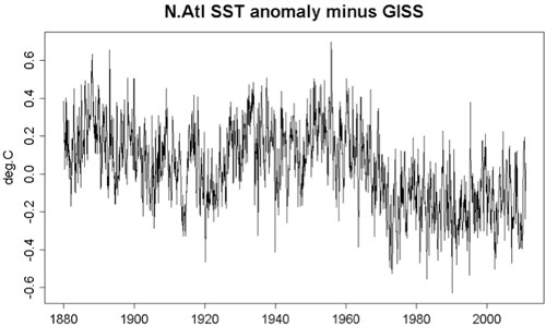
Figure 5: North Atlantic SST minus the global mean.
From a purely technical point, the collinearity introduced between this negative trend in the AMO index and the anthropogenic positive trend confuses the MLR analysis. If you insist on using it, it will give a 50-year anthropogenic trend of 0.1 degree C/decade and a 34-year anthropogenic trend of 0.125 degree C/decade. The 50-year trend is not too much larger than what we obtained previously but these numbers cannot be trusted.
One could suggest, qualitatively, that the negative trend is due to anthropogenic aerosol cooling and the ups and down due to what happens before and after the Clean Air Act etc. But these arguments are similar to the qualitative arguments that some have made about the observed temperature variations as due to solar radiation variations. To make it quantitative we need to put the suggestion into a model and check it against observation. This was done by the HadGEM-ES2 model, and we have discussed above why it has aspects that are inconsistent with observation.
The question of whether one should use the AMO Index as defined by Enfield et al. [2001] or by Trenberth and Shea [2006] was discussed in detail in Enfield and Cid-Serrano [2010] , who argued against the latter index as “throwing the baby out with the bath water”. In effect this is a claim of circular argument. They claimed that this procedure is valid “only if it is known a priori that the Atlantic contribution to the global SST signal is entirely anthropogenic, which of course is not known”. Charges of circular argument have been leveled at those adopting either AMO index in the past, and DumbScientist was not the first. In my opinion, the argument should be a physical one and one based on observational evidence. An argument based on one definition of the index being self-evidently correct is bound to be circular in itself. Physical justification of AMO being mostly natural or anthropogenically forced needs to precede the choice of the index. This was what we did in our PNAS paper.
Enfield and Cid-Serrano [2010] also examined the issue of causality and the previous claim by Elsner [2006] that the global mean temperature multidecadal variation leads the AMO. They found that the confusion was caused by the fact that Elsner used a 1-year lag to annualized data: While the ocean (AMO) might require upwards of a year to adjust to the atmosphere, the atmosphere responds to the ocean in less than a season, essentially undetectable with a 1-year lag. The Granger test with annual data will fail to show the lag of the atmosphere, thus showing the global temperature to be causal.
There is a concern that the AMO index used in our multiple regression analysis is a temperature response rather than a forcing index. Ideally, all predictors in the analysis should be external forcings, but compromises are routinely made to account for internal variability. The solar forcing index is the solar irradiance measured outside the terrestrial climate system, and so is a suitable predictor. Carbon dioxide forcing is external to the climate system as humans extract fossil fuel and burn it to release the carbon. Volcanic aerosols are released from deep inside the earth into the atmosphere. In the last two examples, the forcing should actually be internal to the terrestrial system, but is considered external to the atmosphere-ocean climate system in a compromise. Further compromise is made in the ENSO “forcing”. ENSO is an internal oscillation of the equatorial Pacific-atmosphere system, but is usually treated as a “forcing” to the global climate system in a compromise. A commonly used ENSO index, the Nino3.4 index, is the mean temperature in a part of the equatorial Pacific that has a strong ENSO variation. It is not too different than the Multivariate ENSO Index used by Foster and Rahmstorf [2011] . It is in principle better to use an index that is not temperature, and so the Southern Oscillation Index (SOI), which is the pressure difference between Tahiti and Darwin, is sometimes used as a predictor for the ENSO temperature response. However, strictly speaking, the SOI is not a predictor of ENSO, but a part of the coupled atmosphere-ocean response that is the ENSO phenomenon. In practice it does not matter much which ENSO index is used because their time series behave similarly. It is in the same spirit that the AMO index, which is a mean of the detrended North Atlantic temperature, is used to predict the global temperature change. It is one step removed from the global mean temperature being analyzed. A better predictor should be the strength of the AMOC, whose variation is thought to be responsible for the AMO. However, measurements deep ocean circulation strength had not been available. Recently Zhang et al. [2011] found that the North Brazil Current (NBC) strength, measured off the coast of Brazil, could be a proxy for the AMOC, and they verified it with a 700-year model run. We could have used NBC as our predictor for the AMO, but that time series is available only for the past 50 years, not long enough for our purpose. They however also found that the NBC variation is coherent with the AMO index. So for our analysis for the past 160 years, we used the AMO index. This is not perfect, but I hope the readers will understand the practical choices being made.
Booth, B. B. B., N. J. Dunstone, P. R. Halloran, T. Andrews, and N. Bellouin, 2012: Aerosols implicated as a prime dirver of twentieth-century North Atlantic climate variability. Nature, 484, 228-232.
Chiang, J. C. H., C. Y. Chang, and M. F. Wehner, 2013: Long-term behavior of the Atlantic interhemispheric SST gradient in the CMIP5 historial simulations. J. Climate, submitted.
DelSol, T., M. K. Tippett, and J. Shukla, 2011: A significant component of unforced multidecadal variability in the recent acceleration of global warming. J. Climate, 24, 909-026.
Delworth, T. L. and M. E. Mann, 2000: Observed and simulated multidecadal variability in the Northern Hemisphere. Clim. Dyn., 16, 661-676.
Elsner, J. B., 2006: Evidence in support of the climatic change-Atlantic hurricane hypothesis. Geophys. Research. Lett., 33, doi:10.1029/2006GL026869.
Enfield, D. B. and L. Cid-Serrano, 2010: secular and multidecadal warmings in the North Atlantic and their relationships with major hurricane activity. Int. J. Climatol., 30, 174-184.
Enfield, D. B., A. M. Mestas-Nunez, and P. J. Trimble, 2001: The Atlantic multidecadal oscillation and its relation to rainfall and river flows in the continental U. S. Geophys. Research. Lett., 28, 2077-2080.
Foster, G. and S. Rahmstorf, 2011: Global temperature evolution 1979-2010. Environmental Research Letters, 6, 1-8.
Huang, N. E., Z. Shen, S. R. Long, M. L. C. Wu, H. H. Shih, Q. N. Zheng, N. C. Yen, C. C. Tung, and H. H. Liu, 1998: The empirical mode decomposition and the Hilbert spectrum for nonlinear and non-stationary time series analysis. Proc. R. Soc. London Ser. A-Math. Phys. Eng. Sci., 454, 903-995.
Mann, M. E. and K. Emanuel, 2006: Atlantic hurricane trends linked to climate change. Eos, 87, 233-244.
Trenberth, K. E. and D. J. Shea, 2006: Atlantic hurricanes and natural variability in 2005. Geophys. Research. Lett., 33, doi:10.1029/2006GL026894.
Tung, K. K. and J. Zhou, 2013: Using Data to Attribute Episodes of Warming and Cooling in Instrumental Record. Proc. Natl. Acad. Sci., USA, 110.
Wu, Z. and N. E. Huang, 2009: Ensemble empirical mode decomposition: a noise-assisted data analysis method. Adv. Adapt. Data Anal., 1, 1-14.
Wu, Z., N. E. Huang, S. R. Long, and C. K. Peng, 2007: On the trend, detrending and variability of nonlinear and non-stationary time series. Proc. Natl. Acad. Sci., USA, 104, 14889-14894.
Wu, Z., N. E. Huang, J. M. Wallace, B. Smoliak, and X. Chen, 2011: On the time-varying trend in global-mean surface temperature. Clim. Dyn.
Wunsch, C., 1998: The work done by the wind on the oceanic general circulation. J. Phys. Oceanography, 28, 2332-2340.
Zhang, D., R. Msadeck, M. J. McPhaden, and T. Delworth, 2011: Multidecadal variability of the North Brazil Current and its connection to the Atlantic meridional overtuning circulation. J. Geophys. Res.,, 116, doi:10.1029/2010JC006812.
Zhang, R., T. Delworth, R. Sutton, D. L. R. Hodson, K. W. Dixon, I. M. H. Held, Y., J. Marshall, Y. Ming, R. Msadeck, J. Robson, A. J. Rosati, M. Ting, and G. A. Vecchi, 2013: Have aerosols caused the observed Atlantic Multidecadal Variability? J. Atmos. Sci., 70, doi:10.1175/JAS-D-12-0331.1.
Posted by KK Tung on Tuesday, 7 May, 2013
 |
The Skeptical Science website by Skeptical Science is licensed under a Creative Commons Attribution 3.0 Unported License. |