


 Arguments


The anthropogenic global warming rate: Is it steady for the last 100 years?
Posted on 11 April 2013 by KK Tung
This is a guest post by KK Tung, who requested the opportunity to respond to the SkS post Tung and Zhou circularly blame ~40% of global warming on regional warming by Dumb Scientist.
The observed global-mean temperature has gone through a number of ups and downs since 1850, which is the beginning of the available global temperature record. Our recent paper of Tung and Zhou [2013] in Proceedings of National Academy of Science (PNAS) was the latest among a large body of published literature on the evidence of a multidecadal oscillation that can be seen in the global-mean surface temperature record. We further reported a quantitative analysis (multiple linear regression (MLR)) using the global (not regional) temperature data (HadCRUT4) that attributed a warming rate of 0.07-0.08 °C/decade to net anthropogenic forcing. That warming rate has been steady for the past 100 years, through the ups and downs of about 30-year duration, which we attributed to the Atlantic Multi-decadal Oscillation (AMO). In this view, the anthropogenic warming has not stalled in the past decade and half, nor has it accelerated in the previous three decades. I thank Skeptical Science for giving me this opportunity to explain in a more understandable way some underlying issues that have caused confusion to nonspecialists.
(1) Greenhouse gas concentration vs expected warming
How can the anthropogenic warming be approximately linear in time when we know that atmospheric CO2 has been measured to increase almost exponentially? Implicit in that statement is the expectation that the warming (i.e. the rate of surface temperature increase) should follow the rate of increase of greenhouse gas concentration in the atmosphere. This rather common expectation is incorrect. An accessible reference is that from Britannica.com: “Radiative forcing caused by carbon dioxide varies in an approximately logarithmic fashion with the concentration of that gas in the atmosphere. The logarithmic relationship occurs as the result of a saturation effect wherein it becomes increasingly difficult, as CO2 concentrations increase, for additional CO2 molecules to further influence the ‘infrared window’ (a certain narrow band of wavelengths in the infrared region that is not absorbed by atmospheric gases)”.
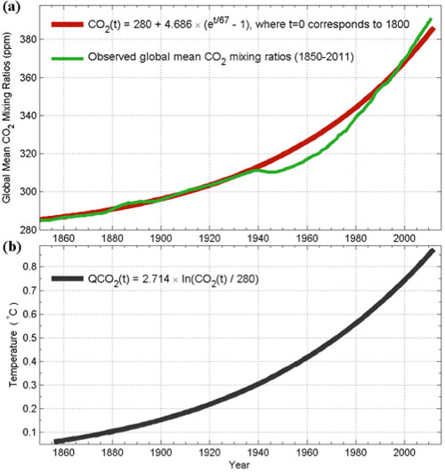
Figure 1. (a) the measured atmospheric concentration of carbon dioxide in green and the fitted smooth function in red. (b) the logarithm of the red curve in (a). The constant multiplier in front converts it to the global mean temperature; details of that MLR analysis are not discussed here to avoid confusion.
Figure 1a shows that the well measured CO2 concentration (in green) can be fitted to an exponential function plus a constant preindustrial value (in red). So it is true that one can claim that the carbon dioxide concentration in the atmosphere has increased at an exponential rate. Normally the logarithm of an exponential function in time is linear in time. However the fit of CO2 has a constant in additional to the exponential, and so its logarithm is slightly more curvy than linear. Nevertheless it can still be regarded as almost linear over multidecadal intervals to within 0.1 °C. Logarithm of that function is shown in Figure 1b as QCO2, which represents the radiative heating from CO2. The exponential growth of the CO2 after 1950 is much muted in the logarithm (taking into account the fact that the vertical scale is in small 0.1°C increments.
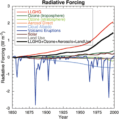
The real situation is more complicated than indicated by these simple functions, because the net anthropogenic forcing is the sum of radiative heatings from individual greenhouse gas concentrations and tropospheric sulfate aerosol cooling (man-made pollution). We show in Figure 2a the sum of radiative heating from all well-mixed greenhouse gases in green and the sum of radiative cooling from tropospheric aerosol effects in blue. Because some of the greenhouse gases such as methane are more powerful radiatively than carbon dioxide, one cannot simply take the logarithm of the sum of the greenhouse gas concentrations to arrive at the total heating rate from them. They need to be calculated individually. These calculated radiative heating rates are available from NASA's Goddard Institute for Space Studies (GISS) at http://data.giss.nasa.gov/modelforce/, and have been used in the GISS model, one of the models participating in IPCC studies. As shown in Figure 2a, the green line is quite nonlinear and shows the acceleration of greenhouse gas forcing after 1950 referred to by DS, but the aerosol cooling also increased after 1950. The net anthropogenic forcing is the small difference of the two large terms. The near cancellation by the two anthropogenic components may be one of the explanations of why the warming deduced by Tung and Zhou is smaller than the response expected from greenhouse gas warming alone. Because the aerosol cooling part is uncertain, we actually do not know what the net anthropogenic forcing looks like. There is no obvious argument that one can appeal to on what the expected warming should be. There is nothing obviously wrong if the anthropogenic warming is found to be almost linear in time. This is the first point I would like to make.
(A side comment: Depending on the exact form of the aerosol cooling adopted, the net anthropogenic forcing is different from model to model. Although you probably cannot see it just by eye-balling the two curves in Figure 2a, their difference actually is nonlinear, with accelerating heating after 1978, allowing the GISS model to produce the accelerated warming after 1978 from anthropogenic forcing alone. Other groups adopt somewhat different time dependent shape of net anthropogenic forcing. See here and here.
Analysis of models by several authors showed that there was a large range of net anthropogenic forcing adopted by models participating in IPCC assessment reports, with a tendency for the models with higher climate sensitivity to adopt a lower net forcing and less sensitive models to adopt a higher net forcing.)
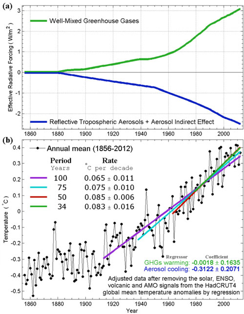
Figure 2. (a) Radiative forcing of various anthropogenic components. (b) Results of Multiple Linear Regression using natural and anthropogenic regressors. Adjusted temperature, which is the same as the combined response to the anthropogenic forcing plus the Residual is shown. This multiple linear regression using two highly collinear regressors is not recommended, but nevertheless yields approximately the same result for the adjusted temperature trend.
(2) “Circular argument”?
One common way to deduce the anthropogenic warming signal from observed data is to remove all other known natural influences, such as El Nino, volcanic aerosols, solar forcing (cyclic and secular) and the AMO. These are called the predictors or regressors. What remains are random climate noise, and the net anthropogenic warming rate. We call the sum of the two the “adjusted data”, following Foster and Rahmstorf [2011] . The MLR model for the observed temperature T(t) is:
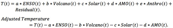
The MLR procedure assumes the form for the predictors and tries to fit the observed temperature with them using the least-squares best fit. The model is successful if the procedure yields a Residual(t) that contains only climate noise, but often it also contains some trend. When that happens it is telling us that the assumed trend in the anthropogenic component (e*Anthro(t)) is probably not correctly giving the anthropogenic trend consistent with the observed temperature.
The adjusted data can be viewed as the temperature with natural variations removed. Because the adjusted temperature can also be expressed as
![]()
the deduced anthropogenic trend can be corrected by adding the trend in the Residual to e*Anthro(t). It turns out that this trend deduced from the Adjusted temperature is not always the same that in e*Anthro(t). This procedure of deducing the trend from Adjusted temperature is actually not sensitive to the assumed form of Anthro(t), as long as it has a long-term trend: When the assumed Anthro(t) has a too large a trend after 1978 compared to before 1978, for example, the Residual (t) will show a negative trend after 1978 and a positive trend before that time. See the example discussed in Zhou and Tung [2013] . Since we do not know a priori what the form of net anthropogenic forcing is because of its large uncertain tropospheric sulfate aerosol component, to be agnostic we used a linear function for Anthro(t) in the intermediate step as a “placeholder”. That was probably the source of the circular argument criticism from DS: “Tung and Zhou implicitly assumed that the anthropogenic warming rate is constant before and after 1950, and (surprise!) that's what they found. This led them to circularly blame about half of global warming on regional warming.” It is important to note that the trend we were talking about is the trend of the Adjusted data, and not the presumed anthropogenic predictor.
We will next show that we get approximately the same result using more nonlinear placeholders for the anthropogenic predictor. In the first example, we proceed to do a MLR analysis using the two anthropogenic predictors: one the nonlinear green line and the other the blue line in Figure 2a, and let the MLR procedure adjust the proportions of the two to get a best fit. This is probably what nonspecialists would find most natural and expect us to do (but specialists know not to do). After the multiple regression analysis is done, the adjusted data is reconstructed by adding the residual to the sum of the two regressed anthropogenic responses. This is shown in Figure 2b. The regression coefficient of greenhouse gas warming is shown as “warming” and the aerosol cooling is shown as “cooling”. The multiple regression analysis is confused by the two highly correlated anthropogenic regressors (this is the well-known problem of collinearity), producing a “warming” that is negative and a “cooling” that is positive. This is not surprising given how close the two curves look in Figure 2a. Nevertheless, the combination of the two responses is robust. When combined to yield the adjusted data, the 100-year, 50-year and 34-year linear trends are still rather steady at ~0.07-0.08°C/decade as shown by the dots in Figure 2b and the trends fitted through them. The result is very close to that found in Tung and Zhou [2013] using a linear predictor as a placeholder. We have tried many other predictors with similar results. Using a nonlinear anthropogenic regressor would still yield an almost linear trend for the past 100 years, if the Residual is added back. And so this procedure is not circular. This is the second point I am trying to make.
Of the different regressors we tried the single anthropogenic regressor that is closest to the final adjusted data turns out to the QCO2(t) function given in Figure 1b. This is shown in Figure 3. The difference between the adjusted data and the QCO2 regressor is the Residual, which is shown in the inset. Except for s a minor negative trend in the last decade in the Residual, it is almost just noise. So the MLR with QCO2 as the anthropogenic regressor is successful. That small negative trend in the Residual, when added back to QCO2, yields a more linear trend in the adjusted data, similar to what we found in Tung and Zhou and in Figure 2b here. (The physical interpretation of why the net anthropogenic warming appears to follow the radiative heating by CO2 alone and with so little lag between forcing and response is rather tricky and will not be discussed here.)
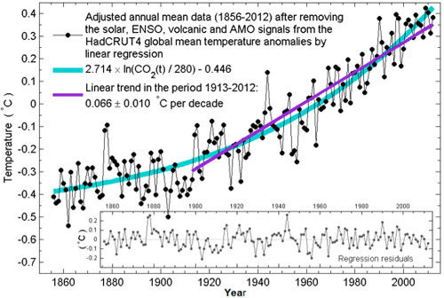
Figure 3. Adjusted data shown in dots, obtained by a MLR using QCO2 as the anthropogenic predictor. The QCO2 is superimposed. The Residual is shown in the inset
(3) “Don’t explain the physics”?
Because of the page limitation of PNAS, a review of the physics of the AMO by other researchers is necessarily brief, with fuller discussions given in the references quoted. Even so, our PNAS paper has the following paragraph on the physical mechanism of the AMO, which Dumb Scientist apparently missed: “The phenomenon likely involves thermohaline circulation variability in the Atlantic Ocean. As described in Dima and Lohmann [2007 ]; Semenov et al. [2010] , the negative feedbacks between the strength of the thermohaline circulation which brings warm sea-surface temperature (SST) to the North Atlantic, and the Arctic ice melt in response to the warm SST, which, because of reduced deep-water formation, then slows the strength of the thermohaline circulation after a delay of 20 years, together create the restoring force responsible for the oscillation. Recently a 55-80-year AMO has been model simulated as arising from the variability of the meridional overturning circulation in the Atlantic Wei and Lohmann [2012] .”
As I have now exceeded the recommended length for the post, I hope in a second post to give a more detailed review of the physical mechanisms of the AMO (noting that the science is not yet settled), its relation to the Atlantic Meridional Overturning Circulation, the choice of the AMO Index (whether the detrending should be point by point or by the global mean), and why the claim that the observed multidecadal variability can be simulated using time-varying aerosols may not be consistent with the observed data.
References
Dima, M. and G. Lohmann, 2007: A Hemispheric Mechanism for the Atlantic Multidecadal Oscillation. Journal of Climate, 20, 2706-2719.
Foster, G. and S. Rahmstorf, 2011: Global temperature evolution 1979-2010. Environmental Research Letters, 6, 1-8.
Semenov, V. A., M. Latif, D. Dommenget, N. Keenlyside, A. Strehz, T. Martin, and W. Park, 2010: The impact of North Atlantic-Arctic multidecadal variability on Northern Hemisphere surface air temperature. J. Climate, 23, 5668-5677.
Tung, K. K. and J. Zhou, 2013: Using Data to Attribute Episodes of Warming and Cooling in Instrumental Record. Proc. Natl. Acad. Sci., USA, 110.
Wei, W. and Lohmann, 2012: Simulated Atlantic Multidecadal Oscillation during the Holocene. J. Climate, doi:10.1175/JCLI-D-11-00667.1.
Zhou, J. and K. K. Tung, 2013: Deducing the multi-decadal anthropogenic global warming trend using multiple regression analysis. J. Atmos Sci, 70, 3-8.


I have two major issues with this response.
My issue with point #1 is that although not all radiative forcing estimates are equal, they do all show an accelerated anthropogenic forcing sometime after 1950, so we should expect to see accelerated anthropogenic warming since, say, the 1970s. If you don't, you have to explain why not, and saying 'the forcing is uncertain' isn't sufficient if all anthropogenic forcing estimates include an acceleration.
My other issue is that the main point of Dumb Scientist's post doesn't seem to be addressed. That's the criticism that AMO is associated with Atlantic sea surface temps, which themselves are warmed by the anthropogenic forcing. So if you remove the AMO influence in your linear regression, you're removing some of the anthropogenic warming, and that may explain why it's apparently underestimated. As far as I can tell, that main point isn't addressed in this response, unless I'm missing it.
Some people are just blinded by science....
Just love the dynamic definition function....
I would agree with dana1981 that the standard AMO index, being a linearly detrended set of sea surface temperatures, is quite tied to global warming and incorporates some of that warming signal - subtracting signal from signal, and reducing the identified anthropogenic component.
Any regression against the AMO requires, of course, defining which AMO index you are discussing - the linearly detrended version, or one as suggested by Trenberth and Shea 2006 Atlantic hurricanes and natural variability in 2005, who recognized the incorporation of a global warming signal into the traditional definition:
Also of interest is Anderson et al 2012, Testing for the Possible Influence of Unknown Climate Forcings upon Global Temperature Increases from 1950 to 2000, which analyzes ocean heat content (OHC), sea surface temperatures, and forcings, and indicates from an energy conservation point of view that:
According to that work, there is insufficient energy available within the constraints of OHC to cause observed warming via natural variability and maintain observed OHC.
Also of note in regards to the AMO definition is Emanuel and Mann 2006, along with a discussion by M. Mann and G. Schmidt at RealClimate, concluding in part that:
[Emphasis added]
Again, subtracting signal from signal is going to give incorrect regression results for other components, and linear detrending is not a good match to the actual forcing history.
Two points regarding Tung and Zhou:
1) If you add a factor to your multiple linear regression, even if it's just random noise, that factor is going to explain some of the trend. If you then put that factor into the non-anthropogenic group, you reduce the anthropogenic part. If the factor correlates with the trend, this effect becomes much stronger. A look at the AMO graph shows that the AMO was at a minimum in 1910, and at a maximum in 2010, which means it is correlating with the trend.
2) Lets take the following model:
T(t) = a * distractor1(t) + b * distractor2(t) + c * distractor3(t) + d * Tdetrended(t) + e * trend(t) + residual(t)
Tdetrended is equal to T(t) with the linear trend removed. trend(t) is the linear trend of T(t). I can already spell out what the best model is: a, b and c are 0, d and e are 1. Taken together, they perfectly reproduce T(t).
This is, in essence, the model of Tung and Zhou. Tdetrended is the AMO, which is defined as the detrended North Atlantic SST. Not quite the detrended world temperature record, but almost. trend(t) is their anthropogenic factor, which they make a linear trend. Because these two factors can explain the temperatures so well, all the other factors become mere distractors.
Note that it does not matter in linear regression which actual trend you use, as long as it is regular. If you would halve trend(t), the factor e would double, and you end up with the same model.
To the degree that NA SST and world temperature correlates, the Tung and Zhou approach can only find linear anthropogenic forcings.
In reply to Dana181: As I said in the last paragraph of the post, I will address the AMO issue in Part 2, which is to come. Dumb Scientists claim of circular argument on our part consists of two parts. The first part deals with the linear regressor used, which is discussed here, and the second part deals with the AMO index used, which will be discussed in my second post.
Concerning Dana181's statement that most models use radiative forcing that show acceleration after 1970s, I just want to make the following observation. The models that adopted the kind of net radiative forcing that varies in time in approximately the same manner as the observed global mean temperature---with cooling in the 1970s and accelerated warming in the 1980s to 2000--were trying to simulate the observed warming using forced response alone (under ensemble average). So the net heating used has to have that time behavior otherwise the model simulation would not have been considered successful. Here we are questioning the assumption that the observed warming, including the accelerated warming in the later part of the 20th century, is mainly due to forced response to radiative heating.
No, I'm not ignoring the last century of physics. It's exasperating to be lectured about the ancient fact that CO2's radiative forcing in Earth's current atmosphere depends approximately on the logarithm of its concentration. My article linked to a graph of CO2's radiative forcing, which accounts for this logarithmic dependence. Notice that CO2's radiative forcing increases faster after 1950, because increasing CO2 faster also increases its logarithm faster. That's what makes the forcing "slightly more curvy than linear".
That same radiative forcings graph also accounts for aerosols. Notice that the black line includes aerosols and also increases faster after 1950.
Perhaps the IPCC's estimates are wrong, but subtracting the standard NOAA AMO index to determine anthropogenic warming is equivalent to assuming that anthropogenic warming is steady before and after 1950. If it isn't, you'll never know because subtracting the AMO will just subtract signal after 1950.
No, that wasn't the source of my criticism. Dana1981, KR and bouke correctly pointed out that your circular argument results from adding the AMO(t) regressor, which is correlated with surface temperatures after 1950 if you used the standard NOAA AMO index.
That's only true for inverse models of aerosol forcings. It's important to note that they're compared to independent forward calculations which are based on estimates of emissions and models of aerosol physics and chemistry.
If you used the AMO index with global SST removed that KR mentioned, then your result is really interesting. I assumed that you used NOAA's linearly detrended N. Atlantic sea surface temperatures, in which case the anthropogenic warming would be hiding in your AMO(t) function. Again, that's because warming the globe also warms the N. Atlantic, and anthropogenic warming was faster after 1950.
It's only circular if you used NOAA's standard detrended AMO index. If so, you added a regressor that's correlated with surface temperatures since 1950. Again, in that case the warming would be hiding in your AMO(t) function.
Dumb Scientist - From Tung and Zhou 2013:
So yes, the paper uses the linear detrended AMO index - which has been indicated by several publications to be in part misidentified global warming.
Dr. Tung promised to discuss "the choice of the AMO Index." Hopefully his discussion will address the fact that the linearly detrended AMO likely contains an anthropogenic trend after 1950. The alternative AMO index you mentioned which is relative to the global mean SST seems like it would be much less likely to mistakenly subtract signal.
KR is right, and I was wrong to manufacture unwarranted doubt by implying that Tung and Zhou 2013 might have used a different AMO index.
Exploring the frontiers of knowledge inevitably results in mistakes. The true test of a scientist is admitting these mistakes and moving on. Especially when the mistake affects the future of our civilization.
So: I was wrong. KR: thank you for correcting me, and for all your other informative comments.
Thanks for your integrity, Dumb Scientist. Looking forward to more insights.
KK Tung @6.
While you are correct to say (as you do) that it is not wrong if net forcing is found to be linear over the period, this is not the same as basing your study on an assumption of net forcing being linear over the period. And given that, I would suggest that it is wrong to not emphasise your reliance on such a linearity and also wrong not to make clear the levels of non-linearity/linearity developed by other people. You acknowledge (but leave us to 'eyeball' your fig 2a rather than properly illustrate it) that GISS conclude there was accelerated heating after 1978 and link to two other graphs in the post. Those two graphs have very significant non-linearity - the SKSci graph of IPCC forcing shows an 8-fold increase in the rate of forcing after the 1960s and it is even more pronounced on the Skeie et al 2011 graph. As for findings of linearity - forgive my ignorance but do you reference any findings of linearity?
Your writing comes close enough to accusing others of creating/exagerating the non-linearity in net forcing solely to support an otherwise unfounded theory (eg "...allowing the GISS model to produce..." "...models to adopt ..." and @6 "...were trying to simulate the observed warming using forced response alone..."), which I consider close enough to be worthy of comment. Are you in any way saying the non-linearity is being exaggerated for non-scientific reasons?
Your comment that warming follows CO2 with such little time lag being rather tricky and "will not be discussed here." I like 'tricky'. Is it to be discussed in a later post? Or is such discussion available elsewhere?
Reply to MA Roger:
While you are correct to say (as you do) that it is not wrong if net forcing is found to be linear over the period, this is not the same as basing your study on an assumption of net forcing being linear over the period.
There was no assumption of net forcing being linear in our work. That was a misunderstanding on the part of Dumb Scientist. In fact, Figure 2 and Figure 3 are two examples using nonlinear net forcing indices. A third example was given in the paper by Zhou and Tung (2013) in Journal of Atmospheric Sciences. It discussed the case of using the nonlinear difference of the two anthropogenic forcing curves displayed in Figure 2a. In all three cases, the deduced anthropogenic response appears rather linear for the past 100 years, as long as one remembers to add back the Residual before measuring the trend.
Your comment that warming follows CO2 with such little time lag being rather tricky and "will not be discussed here." I like 'tricky'. Is it to be discussed in a later post?
It is tricky because it could easily lead to misunderstanding in such a public forum. If CO2 were the only anthropogenic forcing, the response in Figure 3 would have implied that the climate sensitivity is low. However, CO2 is not the only greenhouse gas, and greenhouse gas radiative forcing is not the only anthropogenic forcing. There are some negative anthropogenic forcings, such as tropospheric sulfate aerosols, that subtract from the greenhouse gas forcing. At least that is my current understanding. My previous work, Tung et al (2008), Geophysical Res. Lett., using the observed transient response to the 11 year solar cycle, gives a climate sensitivity estimate that is at the high end of the IPCC range.
My previous comment explained that you are assuming the net anthropogenic forcing is linear, by subtracting the linearly detrended AMO.
Again, as I've already pointed out, that's just because you swept the faster warming since 1950 into the AMO(t) function.
KK Tung @12.
Thank you for clearing up my final enquiry point.
It appears by your reply to my first point that we may be talking at cross-purposes. I will attempt to clarify the point.
My concern here is that most constructions of net forcing in the literature (and as linked in the post) show a strong increase in the net forcing from the 1970s on. Conversely, your paper is proposing a smoother (less bent) increase (described in Tung&Zhou13 as "converging to" a linear trend which to me is highly suggestive of a linear forcing). Neither in this post nor Tung&Zhou13 is the smooth/bent forcing issue adequately addressed.
The two methods presented in Tung&Zhou13, (the 50-y to 90-y wavelet band subtraction & the MLR with AMO index included) expressly attempt to produce a smoother (less bendy) temperature record. Thus when non-linear forcings are fed in (as described in the above post), it is obvious that the profile found "closest to the final adjusted data turns out to the QCO2(t) function", a very smooth forcing profile.
"Finding" a smooth forcing profile is not wrong (your first take-away point). However, such a profile here is the implicit result of your analysis because you began by smoothing the temperature series. It is thus "assumed" and not "found".
I wouldn't go so far to say that this makes for a circular argument. Yet it does require more support for use of a smooth forcing profile as it is "assumed" and to my limited knowledge forcing profiles for the century are usually rather bent. (@11 I also noted a seeming implied view within your post that the "bend" was being unreasonably exaggerated. This is still worthy of comment.)
It should be interesting when the Chinese people demand that the Chinese government stops sending aerosols into the atmosphere. A similar scenario unfolded when America started electrostatically precipitating particulate matter from her smoke stacks and began to scrub out SO2.
I don't understand this point. I thought the issue was simpler, but I might be failing to comprehend in addition to my obvious failure to communicate. Perhaps it would help if we all answered these yes/no questions:
Question 1
Would regressing global surface temperatures against N. Atlantic SST without detrending the SST remove some anthropogenic warming from global surface temperatures?
Yes or no?
Question 2
Now suppose we regress global surface temperatures against N. Atlantic SST after linearly detrending the SST. In other words, we regress against the standard AMO index as Tung and Zhou 2013 did.
Just imagine that anthropogenic forcings increased faster after 1950. In that case, would regressing global surface temperatures against the AMO remove some anthropogenic warming from global surface temperatures after 1950?
Yes or no?
I'll start: my answers are yes and yes. In fact, I think answering yes to question 1 also implies a yes to question 2, but I'm willing to be educated.
Dumb Scientist @16.
The two questions you pose could be answered in a number of contexts with differing assumptions to yield different answers.
But if you add that N.Atlantic SST does contain an AW signal, then the answer to Q1 will have to be yes.
And if you add that the AW signal is not linear, then AMO derived from N.A. SST through linear detrending will still contain an AW signal and the answer to Q2 will have to be yes.
But where do such answers lead? They say 'Yes, they will remove some of the AW signal' and then beg the question 'How much is "some"?' That surely leads off towards the nature of AMO which is the subject of the next part of these posts.
My apologies if the logic I present @ 14 has proved unclear. I shall attempt to re-state it.
If the AW forcing profile is smooth, so too will the AW signal within the temperature record. And visa versa. Thus if an analysis has by its nature the effect of smoothing the AW signal, by its nature it will produce a smooth AW forcing profile. Therefore such analysis cannot in itself be used to show how smooth is AW forcing.
This is perhaps why I spy in the post discontent with bendy forcing profiles - bendy profiles are inconsistent with a significant AMO signal being superimposed on the AW signal.
How could N. Atlantic SST not contain an AGW signal?
Exactly. Such answers would lead to the discussion I wanted to see in Tung and Zhou 2013: namely 'How much is "some"?' I'm astonished that they didn't even address the possibility that they're subtracting signal (unless I missed something?).
As I mentioned to Lee and ptbrown13 in the comments on my article, I have no problem with the idea that AMO variability has parts that are strictly internal and parts which alter the radiative imbalance of the climate. While a discussion of the nature of AMO could be informative, I'm skeptical that the nature of AMO can be elucidated by subtracting AGW after 1950.
In answer to MA Roger at post 14: I am glad I answered your second point. Somehow I still failed to yet my answer through on you're first point. While one of the two methods in Tung and Zhou used smoothing, the second method, the MLR method, does not, and it is this second method that I discussed in the present post. Let me try another way to presenting this point: Give me any nonlinear function that you prefer (within reason of course, and it should have an increasing long term trend), I go through the MLR. I would still get a fairly linear response as long as I add back the residual. The residual compensates for the non linearity of the assumed nonlinear function. We pointed out in Zhou and Tung that it is the removal of the AMO that makes the most difference in getting the final result, a point that Dumb Scientist now correctly understood. It is not the form of the anthropogenic regressor or the amount of smoothing involved. I will talk about the issues related to the choice of the AMO indice in the second post next week. It is not a circular argument.
Dumb Scientist @18
You may call me a pedant if you wish but my reticence to just answering Yes-Yes was more due to philisophy than facts. A question about N.A.SST will involve, as well as our respective understandings of the nature of N.A.SST (which will not be identical, possibly radically so), but also our respective understandings of the nature of the question which also will not be identical, possibly radically so. In this case it was not clear to me if the question was about some hypothetical N.A.SST or the N.A.SST(1856-2013).
KK Tung @19.
I fear you are incorrect. Your answer @12 to the 'first point' did get through. However I disagree with that answer, as I do with what I understand of your renewed answer @19.
May I attempt to explain.
Your two points from the post are
(1) The "finding" of a smooth or even linear net anthoropogenic forcing/warming profile (NAF/WP) is not wrong. I agree, as long as it is a "finding" supported by the data.
(2) The smooth NAF/WP is not the product of circular reasoning. This I pretty-much disagree with as I dispute that the smooth NAF/WP is a "finding." Rather I see it as a product of the analytical method not a product of the data, even using MRL. Because...
We start with a wibbly-wobbly temperature record. We agree that we can see the signature of ENSO and volcanic forcing and if we look the signature of solar forcing too. We are happy that these signatures can be extracted using MLR. This smooths out the wibbly-wobbly temperature record 1980-2011 and we are still happy. If those wibbly-wobbles had been truely part of the NAF/WP then NAF/WP would look more the product of a hyper-active child armed with graph paper and crayon than the product of climatological analysis.
In Tung&Zhou13 this MLR is carried out 1850-2011 which yields a profile not dissimilar to the temperature record for 1850-1980, a bendy profile, perhaps an oscillating profile. This we are agreed should contain all the NAF/WP.
Now the 1850-2011 profile (before and after extracting ENSO etc) is remarkably similar to the AMO profile. If you remove that AMO profile, because of that strong similarity, you will always get a smoothed result. If this smoothed result contains the full NAF/WP, the NAF/WP will arguably be likewise smoothed. This is not a "finding" of the analysis. It is the natural outcome of the process. It can be no other way given the choise of using AMO.
The "finding" is not a smooth NAF/WP but if it is legitmate to extract the AMO profile and leave the full NAF/WP behind, the corollary (no stronger) is that NAF/WP will be smooth.
There are parts @19 which I struggle with, although this may be pre-empting the next post.
You say "The residual compensates for the non linearity of the assumed nonlinear function." Yet you describe in the post how you treat that Residual. You proclaim your analysis "successful" because "Except for s a minor negative trend in the last decade in the Residual, it is almost just noise." Surely reducing the Residuals to almost just noise and calling it "successful" leaves no room for any non-linear function, NAF/WP or otherwise.
I wasn't planning to call you anything. In fact, I think your responses have been quite helpful. For the record, I was referring to the same N.A.SST(1856-2011) used in Tung and Zhou 2013, which do contain an AGW signal.
I've repeatedly pointed out that the form of the anthropogenic regressor or adding the residual back is not the problem that concerns me. It's the fact that warming the globe also warms the N. Atlantic, and that net anthropogenic warming was faster after 1950.
I still think it's circular to subtract a linearly detrended AMO to determine AGW, and then find that the remaining AGW is linear. I've been consistent about this point for months, so it's not clear what I "now correctly understood" because that seems to imply a shift in my understanding that I'm not aware of.
I'm grateful to MA Rodger for answering my two yes/no questions. Dr. Tung, would you please answer them? It would only take a few seconds, and I'm very interested to see what your answers will be. Thank you for your time.
In answer to MA Roger at post 21: Now we are getting to the point! Please read our paper, Tung and Zhou. MLR is a mathematical procedure, not a physical one. In our paper it came towards the end after evidence---and there were many pieces----was presented that supports physically the need to remove the AMO to reveal the anthropogenic response. Then we said, "Now we are in a position" to do this quantitative analysis, which is the MLR. You would be right if all we did were to see an AMO-like bent in the data and we removed that. Someone else may disagree with the evidence that we presented and have a better argument for removing the Pacific Decadal Oscillation, for example. Then he/she would then do a MLR using the PDO as a regressor. This is the scientific process. Neither is circular. I would accept his/her MLR result over mine if I find his physical argument and observational evidence presented more compelling.
On your last point. Consider the case of a time series--let's use it as the observation----that contains a nonlinear "anthropogenic " signal and a white noise. And nothing else. Suppose the noise is large and I can't see the anthropogenic signal without doing the MLR analysis, but I do not know what to use for the anthropogenic regressor. So I have to guess. Now suppose I am lucky and chose a regressor that happens to be varying in time like that nonlinear signal. After doing the MLR the residual is found and I examine that carefully. I see that it is white noise. The conclusion I would then make is that the MLR is successful and the anthropogenic signal is nonlinear. If on the other hand I am unlucky and picked a linear function as my regressor, then the residual will not be just noise, but have some trends as well. Then I would conclude that my MLR is not successful and the anthropogenic signal should be nonlinear. Then for my second try I would pick a more nonlinear regressor, until the residual becomes just noise.
I haven't read everything through (boy, you guys are long-winded), but I think to me the crux of the problem is "how much of AMO is inherent in AMO, and how much of AMO is a response to rising temperatures?"
To put it another way, ENSO events can be measured by using observations other than temperatures... sea surface height, barometric pressure differences, and even sea surface temperature distribution (i.e. is the east markedly different from the west). One can measure ENSO events (if one wishes) based on criteria which have nothing to do with absolute temperature changes, and so one is able to separate those two components.
By measuring AMO purely using temperatures, no matter what you do, you are unable to separate cause and effect. No argument is of any meaning unless and until you come up with a measure for AMO that is independent of temperature.
For example, KK Tung says in his post:
Is it possible to describe an AMO index which is based entirely on some (non-temperature based) strength of the thermohaline circulation, and so to correlate the AMO itself with temperature changes rather than correlate temperature changes to temperature changes?
Dr. Tung:
Please consider all the comments about the inclusion of temperature in the calculation of AMO - this is an issue that is important. ENSO has been mentioned in this context, as a phenomenon that can be defined without using temperature as part of the calculation (e.g. here).
Note that ENSO, meaning El Nino - Southern Oscillation is made up of two phenomena that were identified independently before they were recognized as being related. The Southern Oscillation Inex (SOI) was originally identified solely from the pressure difference between Tahiti and Darwin, and it was recognized that it varied over time and could be related to weather changes. El Nino was a phenomenon related to ocean temperatures (and its effect on weather and fishing off the coast of S. America) Only later was the physical link between the two recognized and explained (and research continues). The fact that SOI can be calculated without measurements of T is important - even if the pressure is related to T through atmospheric dynamics, there is an independence of SOI as a numerical value from any T results you want to look at.
In a T=f(x, other terms) situation, you need to be sure that your arrangement of terms doesn't have you looking at a T=f(x)*f(T) situation. What people are suggesting is that you have phrased things as T=f(x)*f(AMO) + other terms, but because f(AMO) includes an f(T) component, you are not properly isolating T on the left side of the equation. Writing the equation as f(AMO) only hides the fact that you are writing T=f(T) - a substitution of the AMO=f(T) relationship shows clearly that you have a T=f(T) equation.
It might help if you can provide part II of your response soon - that may help focus the discussion.
KK Tung @23.
You say I "would be right if all we did were to see an AMO-like bent in the data and we removed that." (The likeness between N.A.SST & global temps is of course stark and easily seen.) Your statement appears to show we are here in accord - the "finding" of a smooth anthropogenic signal is absent if "all we did were to see an AMO-like bent in the data and we removed that." Thus the "finding" lies in that other doings, and is thus the subject of future post(s).
If so, it does lead back to the crux of the initial point @11. In Tung & Chou 2013 you describe as competing 'theories' on the one hand the work you present (within which the smooth anthropogenic signal described mathematically as a log function of CO2 is considered "successful") and on the other the more common "theory that the observed multi-decadal variability is forced by anthropogenic aerosols" (within which the bent anthropogenic signal is employed eg IPCC or Skeie et al fig 1c).
Is it thust your opinion that the two signal profiles (smooth & bent) are also "competing"? (It was my contention @11 that this 'competition' should be explicitly part of the debate and it would be wrong if it were not so.)
(I should also make clear that I am here uncomfortable in expressing Tung & Chou 2013 & IPCC AR4 2007 as theoretically equivalent.)
Gentlemen:
I do not pretend to follow all of the agument threads contained here, but despite my best efforts I have not seen one question that struck me addressed.
Doctor Tung states:
The real situation is more complicated than indicated by these simple functions, because the net anthropogenic forcing is the sum of radiative heatings from individual greenhouse gas concentrations and tropospheric sulfate aerosol cooling (man-made pollution).
Correct me if I am wrong, but isn't there a difference in persistence in the atmosphere amounting to at least one, and possibly two orders of magnitude between sulphate areosols and greenhouse gases? As william points out, even the Chinese have a limit on what they are willing to tolerate in terms of air pollution, so what happens when those two trend lines start to diverge?
On a side note, am I correct in assuming that greenhouse gases are mixed in the atmosphere more uniformly than sulphate areosols are? Could the regional effects of aerosols (presumably greatest closest to their source) on the surface temperatures in the Western Pacific be in any part responsible for the chilliness of the ENSO cycle so far this century?
Best wishes,
Mole
Replying to post 27: Yes, that is the main takeaway. The aerosol residence times are short, and so if China and other developing countries decide to clean up their air, the net anthropogenic withalwithal go up very quickly.
Replying to post 26: They are all competing net heating profiles in the sense that they all lie within the range of uncertainty of aerosol cooling stated in IPCC AR4.
KK Tung @28.
You say "...they all lie within the range of uncertainty of aerosol cooling stated in IPCC AR4." I have never seen such a statement of uncertainty within IPCC AR4. The best I can find is in 2.9.5 Time Evolution of Radiative Forcing and Surface Forcing - "As for RF, it is difficult to specify uncertainties in the temporal evolution, as emissions and concentrations for all but the LLGHGs are not well constrained."
This strongly suggests no such quantified range is defined. Is it possible for a pointer to the statement you reference? It is possible you are inferring the 'Time Evolution' profile uncertainty (ie how bent, how smooth) from the widely known uncertainty presented within IPCC AR4 for at a single date in time (eg the year 2000).
The sense of the word "competing" I used was actually taken from Tung&Chou13 to mean as well as being in the same contest, also in conflict with each other (that is not in the same team), the latter being absent from your use.
You say of multi-decadal wobbling of the global temperature record in Tung&Chou13 "If it is interpreted as natural and related to the Atlantic Multidecadal Oscillation (AMO), then the trend attributed to anthropogenic arming should be significantly reduced after 1980, when the AMO was in a rising phase. However, if it is forced by time-varying aerosol loadings, it should properly be interpreted as part of an accelerating anthropogenic trend. We argue that the former is true, using information from the preindustrial era."
You seem to be reluctant to affirm the position that the smooth forcing profile is consistent only with "the former" and the bent forcing profile only consistent with 'the latter'.
Can you affirm this? Or otherwise, can you indicate the reason it cannot be?
Just as a brief addition to what's already been said. As MA Rodger has mentioned, the anthropogenic forcing time serie published in Skeie et al. (2011) shows strong multidecadal variability (Fig.1c). I consider it superior to any other forcing estimate. Given the highly non-variable nature of the imposed forcing, your assumption of internal variability breaks down. To illustrate the temporal coincidence, I plotted the surface temperature of North America, Europe (GISS), and North Atlantic(HadSST2) vs. anthropogenic and volcanic sulfate forcing (plus OHC):
For the chosen domains see here. North America and North Atlantic nicely agree. Note the perfect agreement between sulfate forcing and temperatures. It is certainly not just coincidence, as the same (short term) response can be seen for volcanic forcing. Given the nature of the circulation (jetstream blowing from west to east), the ocean just follows the atmospheric temperatures, as Tamino pointed out at his blog. On top of that, land temperatures seem to lead the AMO as Tamino also pointed out. If you subtract the GISS NH from North Atlantic temperatures, you get this:
This is the true AMO signal which remains.
The one thing I found really surprising in your paper was how easily you rejected Booth et al. (2012). Overestimation of the aerosol forcing (as nicely argued from Zhang et al. (2013)) does not make it go away. If you take the strong volcanic activity around 1815-1840 and 1880-1910 together with the anthropogenic sulfate forcing between 1950-1970, you can explain three distinct cycles. You mentioned another one between 1660-1680. Makes it four cyles. The frequency coincides with the spectral peaks between 60-90 years. No surprise that you just found that (as others did before). May very well be pure pseudo-oscillatory behavior.
Finally, how do we know that the sulfate forcing is real? We have measured it!
(1) The downwelling SW (clear sky) radiation was reduced, known as global dimming and later brightening (see Skeie (2011) or Wild (2012)).
(2) The anthropogenic sulfate aerosols are clearly identifiable even in Arctic ice cores (graph taken from Tamino). It must have affected NH temperatures!
I wonder why you carefully omitted the discussion of these aspects in your paper? To be honest, I personally can't see how your paper contributes in any way to advance our understanding. Given the aforementioned shortcomings, I consider your paper not only a pointless curve-fitting exercise which does not tell me anything about proper attribution, I consider it to be simply wrong. Perhaps you can offer some more compelling evidence in your second post ... which I am looking forward to. I finish with two papers which I found much more convincing: Ottera et al. (2010) and Terray (2012). They both made a nice effort to disentangle the different drivers at play.
So that I don't appear as impolite for not answering questions on the AMO, just want to say that I had submitted my second post on Tuesday, and it is awaiting its turn at SkS.
Dr. Tung:
No problems. It makes sense to spend time preparing the second post, rather than trying to answer questions that people are asking because they haven't yet seen the second post.
Thanks for taking the time to prepare this, and for participating in the discussion.
Dr. Tung - I would also like to express my appreciation for the very interesting discussion.
Dr Tung, although one might receive my above comment (#30) as destructive (if not offensive), I'd like to stress that I merely expressed my personal opinion ... unfortunately in a rather dismissive and brisk tone for which I humbly apologize. I am just too tired of all these unconvincing attempts to blame the AMO for everything. As I said, I am looking forward to the second post (which is certainly gonna be up soon).
Replying to KR: Thank you for the comments. I appreciated the opportunity to discuss the various issues involved.
Due to my inexperience, I have found it difficult to answer individual questions, mostly of them are technical in nature. I have tried to explain the technical details, but that did not seem to work. Now I appreciate why Gavin Schmidt in Realclimate.org won a prize for communication.
A general comment not related to any post in particular: There is no obviously right or wrong answers; this is always the case when the science is unsettled---when the science is settled I will have to move to another field. One argues for the reasonableness of the assumption using evidence and physical mechanisms, and then proceeds to deduce what that assumption will lead to as consequences. In scientist publications, one always lists the assumption clearly so that others could refute it. We should argue whether the assumption is supported by the available evidence or not. But claiming that the argument is circular simply based on the technical fact that the consequence arose from the assumption is missing the bulk of the arguments in our paper leading to that assumption. I suspect a lot of that may have to do with the fact that our paper is behind a "pay wall", so that many posting here may not have read more than the abstract. I have posted a free link to the entire paper in the first few lines of my post.
A correction: The link to our PNAS paper was deleted in this first post. I hope it survives in my second post, where it is provided again.
It didn't work because your technical details didn't address my point, as many have noted above. That's why I distilled my point into two yes/no questions. I look forward to the educational answers you've undoubtedly provided in your second post.
Science can be (loosely) defined as the search for answers which are less wrong than previous answers. That slogan is meaningless because all science has uncertainties.
It's true that all science is based on assumptions, such as conservation of energy. But no study based on the assumption of energy conservation would conclude that energy is conserved. That would be a circular argument.
You regressed global surface temperatures against the AMO in order to determine anthropogenic warming. Because the AMO is simply linearly detrended N. Atlantic SST, this procedure would only be correct if AGW is linear. Otherwise you'd be subtracting AGW signal, sweeping some AGW into a box you've labelled "natural" called the AMO. So you're assuming that AGW is linear, and you're also concluding that AGW is linear.
Actually, the first link in my article was a free link to the entire paper Tung and Zhou 2013.
Dr. Tung, I'd also like to thank you for your participation here. Right now I'm also trying to explain Antarctic ice mass balance at Jo Nova's, and the disappointing responses made me appreciate this civilized discussion even more.
Nice work DS
I couldn't even show her the difference between a negative temperature trend and 'statistically significant cooling'.
While we are awaiting KK Tung's second post, it may be worth considering what the thesis presented by Tung & Chou 2013 ought to be establishing.
Here in this post, the consequence presented by the thesis was that of the 'flat' forcing profile. Although no supporting evidence for such a 'flat' profile has been offered, our inability to quantify negative forcings with any useful accuracy does not preclude such 'flatness'. Perhaps the strongest argument that it may be 'flat' is the rise in global temperatures 1910-1940. Attributing natural or human forcing to this rise has not been entirely convincing leaving the door open for T&C13 to suggest natural variation as a cause while pointing at the AMO as chief suspect.
Myself, I am tempted to suggest that the human input remains yet to be fully researched. For instance, 1910-40 was overwhelmingly fuelled by coal yet it also saw the rise of the electrical grid which as today must surely have greatly impacted the levels of pollution per ton of coal burnt. Such consideration I have not seen mentioned for early 20th century climate forcing.
The second post we eagerly await will presumably lead to discussion of the proportion of AGW present within the AMO signal (and the flip-side of that - how much AMO is present in the global temperature record). This does need to be fully addressed to prevent accusations of curve-fitting.
Yet I don't think that is the primary requirement for T&C13. The thesis stands more strongly than say Asakofu (which is simple curve-fitting). T&C13 does more than just assert that the global climate, as exemplified by the AMO, is ringing like a bell and that it has done so for the last few centuries. T&C13 presents evidence for this 'ringing bell'. If compelling evidence for the 'ringing bell' exists, it doesn't really matter if it is driven by AMO, PDO, ENSO, AO or smelly BO.
It is thus evidence of the 'ringing bell' that I consider the most important question, be it within AMO reconstructions or the CET record.
DS @7: You said, "increasing CO2 faster also increases its logarithm faster"
I believe this assertion is false, because increasing CO2 faster does not necessarily increase its logarithm faster. By "increasing CO2 faster" I take you to mean that as time marches on, the first derivative of CO2 as a function of time increases, i.e., the second derivative is positive. Thus, I take your assertion to be that if the the second derivative CO2 as a function of time is positive, then the second derivative of the logarithm of CO2 as a function of time must also be positive. If this understanding of what you are asserting is correct, then what you are asserting is false.
As a simple counterexample, let's say CO2 = t2.
t2 is a function that "increases faster" over time, i.e., its first derivative, 2t, increases as t increases, and its second derivative, 2, is positive.
Therefore, if your statement that "increasing CO2 faster also increases its logarithm faster" were true, then the first derivative of ln(t2) should also increase as t increases.
Let's have a look to see if it does:
d ln(t2)/dt = d ln(f)/df * d(t2)/dt, where f = t2 (applying the chain rule)
=> d ln(t2)/dt = (1/f) * 2t = (1/t2) * 2t = 2/t, which decreases as t increases. (I.e., differentiating again to get the second derivative, you get -2/t2 which is negative for all real values of t)
So your broadly stated assertion is false.
Even if we take the example of CO2 being equal to (or proportional to) et, which has a positive second derivative (the first derivative of et is itself, as is the second derivative), the second derivative of ln(e^t) = d2ln(e^t)/dt2= d2t/dt2 = d(1)/dt = 0. In other words, even an exponential relationship of CO2 to time tends to result in a linear relationship between temperature and time. A linear relationship is what the Tung study apparently found, which is not inconsistent with the understanding that emissions are rising exponentially, assuming a simple relationship where temperature change is proportional to the logarithm of CO2 change.
This is not to say that there are no examples of f(t) having d2f(t)/dt2 > 0 where d2(ln(f(t))/dt2 is also > 0. (For example, if CO2 = et^2, read "e to the t squared" then the second derivative of CO2 and the second derivitive of its logarithm would both be positive.) But that's not the same as saying the former implies the latter, which is how I read your premise, on which you apparently based your conclusion that Tung's interpretation of the data was aphysical.
Don't get me wrong, I know next very little about the physics, but based on my understanding of calculus, I suspect you had overlooked this nuance of the math.
Heh, I just noticed that I applied the chain rule to differentiate ln(t2) instead of just convering it into 2ln(t) and differentiating that - shows my own math is a little rusty... But it doesn't change the result of the second derivative, -2/t2
jdixon1980 - The logarithm of a number increases (logarithmicly) as the number increases, the log decreases as a number decreases. That's by the definition of a logarithm.
If CO2 is rising at eT*N, then speeds up to eT*(N+1) the natural log rise rate will go from T*N to T*(N+1). In other words, if CO2 rises faster over time, the forcing (the log of CO2 change) will also rise faster over time.
I suggest you check your math - time is not the base, it's a multiplier in the exponent.
jdixon1980 - Not incidentally, Tamino demonstrated some time ago that CO2 is in fact rising faster than exponentially, hence CO2 forcings are rising faster than linearly.
[Source]
KR @42, 43 - thanks for the clarification that time is a multiplier in the exponent. I don't think that's a sign of my needing to check my "math" per se, so much as my (lack of) knowledge of the actual relationship of CO2 rise to time. My math is consistent with what you are saying - in your example where a function that is initially e^(T*N) subsequently becomes e^(T*(N+1)), it may be that the constant term in the exponent changed from N to N+1 because it is not actually a constant, but a linear function of time, which would give you something that acts like e^(t^2), an example that I mentioned of a situation in which a function "increases faster" as its logarithm also "increases faster."
However, I assume you are suggesting that the second term is not actually a linear function of time, but rather a step function that abruptly shifted being a constant N to a constant N+1, at some precise moment or over some short interval, because of some historical event causing an abrupt shift in the emissions trend? As you illustrate, DS's statement would hold true for that case as well, because as you illustrated the first derivative of the logarithm would change from N to N+1.
I hadn't considered this kind of abrupt shift when trying to understand and evaluate DS's statement. I still would contend that not all abrupt transformations of a function resulting in a transformed function having a larger first derivative would also result in a logarithm of the transformed function having a larger first derivative; for instance it wouldn't hold true if CO2 = (N)t^2 suddenly became CO2 = (N+1)t^2, but that's just a quibble with his wording that I wouldn't have brought up had I initially understood the context, which I do now thanks to your clarification.
jdixon1980 - While I used N and N+1 for illustration, there hasn't been a sudden abrupt shift, but rather (as seen in the CO2 data) an increase in the rate of CO2 increase rising over time, a positive second derivative. And a fairly simple check on this, taking the ln(CO2) and looking at its behavior over time, shows that forcing is actually increasing greater than linearly, that CO2 is increasing greater than exponentially.
Abrupt or not, if CO2 concentration shows a faster increase over time, the Ln(CO2) will also show a faster increase over time.
KR @45 "Abrupt or not, if CO2 concentration shows a faster increase over time, the Ln(CO2) will also show a faster increase over time." This broad mathematical proposition is false, as I showed above by the counterexample in which CO2 = t^2. But the point is moot because, as you point out, we can see from observation that ln(CO2) actually is increasing faster over time. I know that now, because you pointed it out to me, though it wasn't clear to me from DS's statement at 7. The reason why the mathematical proposition holds true in for the particular case of CO2 as a function of time is that CO2 apparently is not proportional to t^2, or for that matter even to e^t (the second derivative of ln(N*e^t) being zero, not positive), but to something even higher order than that.
SkS is good for people like me who are technically literate (I'm a patent attorney with a mechanical engineering degree, which is admittedly growing stale after ten years) but lack broad climate knowledge, precisely because of instances like this: I read something that confuses me by contradicting what I remember from first-semester calculus, I comment about it, and someone like you can straighten me out by explaining the context that makes sense of the confusing statement, in this case by showing me that the confusing statement wasn't intended as broadly as its literal reading.
For a reality check, I asked my friend Lucas about it (a math professor and a Climate Reality Leader with the Climate Reality Project). Some of his reply went a little over my head on a quick reading, but the gist of it is that whether increasing the first derivative of a function will also increase the first derivative of its logarithm depends on what the function is:
"J: Just because a function's derivative is increasing doesn't mean the derivative of the log of the function is increasing. For a function's log to have increasing derivative, it must satisfy a certain differential equation: d^2(ln(f))/dt^2 = (f(t)f''(t)-(f'(t))^2)/f^2(t) > 0 <=> f(t)f''(t) > (f'(t))^2. This is never true for lines (f''(t) = 0) and typically not true for polynomials (for a polynomial with leading term x^n, the leading term on the left is n(n-1)x^(2n-2) and the leading term on the right is n^2x^(2n-2), so the right always eventually dominates).
However, I'm not sure that's what DS meant. DS might mean that if you increase the first derivative of f then you also increase the first derivative of ln(f). More formally, if f(0) = g(0) and f'(t) > g'(t) for t > 0 then (ln(f(t)))' > (ln(g(t)))' for t > 0. Even this might not be true though. For it to be true, we would need the following differential equation to hold: (ln(f(t)))' = f'(t)/f(t) > g'(t)/g(t) = (ln(g(t)))', or equivalently f'(t)g(t) > f(t)g'(t). This now holds true for lines (if f(t) = at+f(0) and g(t) = bt+f(0), the differential equation is abt+af(0) > abt+bf(0), which is true exactly when f'(t) = a > b = g'(t)). It is also true for pure exponential functions (if f(t) = a^t and g(t) = b^t then the diff eq becomes ln(a)a^tb^t > ln(b)b^ta^t, which is true iff a > b iff f'(t) > g'(t)). But for more complicated functions, the exact relationship depends on the functions involved."
jdixon1980 - What DS said:
Now if CO2 were increasing in a polynomial fashion, its log (while still increasing with CO2 - the log of a larger number is larger than the log of a smaller number), would by definition have a positive first derivative, but would have a negative second derivative - less than exponential growth, less than linear forcing increase. If that polynomial grew larger (faster growth curve), the log would increase faster than it would otherwise have, with a higher (although potentially still negative) second derivative.
In the case of actual CO2 measures, the growth of CO2 is higher than exponential, the log of CO2 has positive first and second derivatives. DS did skip a step, though, and did not mention that CO2 growth is faster than exponential.
But no matter what, if the rate of growth of a value increases, the growth of the log of that value (always with a positive first derivative under growth) will grow faster than it would without that increase.
Dr. KK Tung - You stated that "atmospheric CO2 has been measured to increase almost exponentially".
This is incorrect, CO2 is increasing more than exponentially over the last century, and the CO2 portion of forcings is therefore increasing faster than linearly.
It will be interesting to see Dr. Tung's response to KR@49, assuming that Dr. Tung's conclusion rests on the premise that CO2 is increasing "almost exponentially" as opposed to "more than exponentially."