Climate Science Glossary

Term Lookup

Enter a term in the search box to find its definition.

Settings

Use the controls in the far right panel to increase or decrease the number of terms automatically displayed (or to completely turn that feature off).

Term Lookup

Settings


All IPCC definitions taken from Climate Change 2007: The Physical Science Basis. Working Group I Contribution to the Fourth Assessment Report of the Intergovernmental Panel on Climate Change, Annex I, Glossary, pp. 941-954. Cambridge University Press.

Home Arguments Software Resources Comments The Consensus Project Translations About Support

Bluesky Facebook LinkedIn Mastodon MeWe

Twitter YouTube RSS Posts RSS Comments Email Subscribe


Climate's changed before
It's the sun
It's not bad
There is no consensus
It's cooling
Models are unreliable
Temp record is unreliable
Animals and plants can adapt
It hasn't warmed since 1998
Antarctica is gaining ice
View All Arguments...


Username
Password
New? Register here
Forgot your password?

Latest Posts

Archives

Simply Wrong: Jan-Erik Solheim on Hansen 1988

Posted on 19 June 2012 by dana1981

The myth that Hansen's 1988 prediction was wrong is one of those zombie myths that always keeps coming back even after you chop its head off time and time again.  The newest incarnation of this myth comes from Jan-Erik Solheim, who in a 272 word article promoted by Fritz Vahrenholt and Sebastian Lüning (translated by the usual climate denial enablers here) manages to make several simple errors which we will detail here.

Whopping Wrong Temperature Change Claim

Solheim claims that "Hansen’s model overestimates the temperature by 1.9°C, which is a whopping 150% wrong."  Yet Scenario A - the emissions scenario with the largest projected temperature change - only projects 0.7°C surface warming between 1988 and 2012.  Even if emissions were higher than in Scenario A (which they weren't, but Solheim wrongly claims they were), they would have to be several times higher for Hansen's model to project the ~2.3°C warming over just 23 years (1°C per decade!) that Solheim claims.  Solheim's claim here is simply very wrong.

CO2 is Not the Only Greenhouse Gas

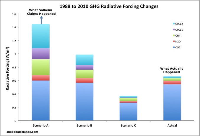
Quite similar to Patrick Michaels' misrepresentation of Hansen's study back in 1998, Solheim claims that Hansen's Scenario A has been closest to reality by focusing exclusively on CO2 emissions.  However, the main difference between the various Hansen emissions scenarios is not due to CO2, it's due to other greenhouse gases (GHGs) like chlorofluorocarbons (CFCs) and methane (CH4), whose emissions have actually been below Scenario C (Figure 1).  In fact, more than half of the Scenario A radiative forcing comes from non-CO2 GHGs.

solheim vs reality

Figure 1: Radiative forcing contributions from 1988 to 2010 from CO2 (dark blue), N2O (red), CH4 (green), CFC-11 (purple), and CFC-12 (light blue) in each of the scenarios modeled in Hansen et al. 1988, vs. observations (NOAA).  Solheim claims the actual changes were larger than Scenario A (indicated by the blue arrow).  In reality they were smaller than Scenario B.

Wrong on Temperature Data

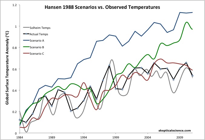
Solheim also produces a very strange plot of what he claims is "the ultimate real-measured temperature (rolling 5-year average)."  His plot shows the purported 5-year running average temperature around 1998 as hotter than at any later date to present, which is not true of any surface or lower atmosphere temperature data set. It appears that Solheim has actually plotted annual temperature data, or perhaps a 5-month running average, most likely from HadCRUT3, which has a known cool bias and has of course been replaced by HadCRUT4.  There is simply no reason for Solheim to be using the outdated data from HadCRUT3.

Figure 2 shows what the comparison should look like when using the average of HadCRUT4, NASA GISS, and NOAA temperature data sets.

Hansen vs Obs vs Solheim

Figure 2: Hansen's 1988 Scenario A (blue), B (green), and C (red) temperature projections compared to actual observed temperatures (black - average of NASA GISS, NOAA, and HadCRUT4) and to Solheim's temperature plot (grey).

Wrong Conclusion

Ultimately Solheim's concluded "The sorry state of affairs is that these simulations  are believed to be a true forecast by our politicians."  However, even if global climate models from several decades ago didn't have the remarkable record of accuracy that they do, current day clmate modeling is far more sophisticated than that done by Hansen et al. nearly a quarter century ago.  Climate models are now run on some of the world's fastest supercomputers, whereas Hansen's was run on a computer with substantially less computing power than a modern day laptop.  While climate model forecasts are imperfect (as are all forecasts), they have thus far been quite accurate and are constantly improving.

What Can We Learn From This?

The observed temperature change has been closest to Scenario C, but actual emissions have been closer to Scenario B.  This tells us that Hansen's model was "wrong" in that it was too sensitive to greenhouse gas changes.  However, it was not wrong by 150%, as Solheim claims.  Compared to the actual radiative forcing change, Hansen's model over-projected the 1984-2011 surface warming by about 40%, meaning its sensitivity (4.2°C for doubled CO2) was about 40% too high.

What this tells us is that real-world climate sensitivity is right around 3°C, which is also what all the other scientific evidence tells us.  Of course, this is not a conclusion that climate denialists are willing to accept, or even allow for discussion.  This willingness to unquestioningly accept something which is obviously simply wrong is a good test of the difference between skepticism and denial.  Indeed, in misrepresenting Hansen's results, Solheim has exhibited several of the 5 characteristics of scientific denialism.

0 0

Printable Version  |  Link to this page

Comments

Prev  1  2  

Comments 51 to 77 out of 77:

  1. Consider Hansen 1988 as a piece of advice to policy makers and investors. The advice was that different emission regimes would result in different levels of warming over the next several decades. Importantly, he advised that the temperature difference between A) Continued exponential GHG growth and B*) An emissions plateau by 2000, could be as much as 0.8C by 2019. Was this bad advice? No. Although following his advice would have resulted in a carbon price that was too high, it would have been a lot more accurate than its actual price in 1988, which was $0.00.
    0 0
  2. Forgot my addendum! *Note that my 'B)' is Hansen's 'Scenario C', lest there be any confusion.
    0 0
  3. angusmac - climate sensitivity did not fall, the sensitivity in Hansen's climate model "fell". Climate sensitivity has always been around 3°C. You still seem entirely focused on "Hansen was wrong", in which case I again refer you to the final section in the above post.
    0 0
  4. angusmac maybe needs to go back and read Hansen 1988 again. Hansen specifically states that even then the NAS had concluded climate sensitivity was likely around 3C.
    0 0
  5. dana, by pixel count, temperature anomaly that Solheim claims would have been predicted with actual forcings is 18% higher than that for scenario A. In contrast, you only show him as showing a forcing 9% greater than that in scenario A. Curiously, if you apply a 2.5% increment to the growth of CO2 from 1951 in a manner similar to that described in Appendix B of Hansen et al, 88, the result is an 18% greater increase of CO2 concentration from 1981 to 2011 than is shown in Scenario A. This strongly suggests that Solheim has not only applied the 2001-2011 growth rate of CO2 over the entire period of the projection, despite the well known fact that growth in CO2 concentrations was much reduced in the 1990s, but that he has also treated CO2 as the only forcing. It is not certain that that is what he has done, but it is the simplest explanation of his error. As it happens, in assuming that he took a more reasonable approach, you appear to have underestimated his error.
    0 0
  6. Tom - Solheim's figure was entirely unclear to me. I couldn't tell if his arrow was intended to stop at the supposed actual forcing-corresponding temperature change, or if it was just pointing in that direction. Given that he said the model overestimates the temperature by 1.9°C, I just couldn't figure out what he was trying to show in that figure. The arrow didn't indicate a 1.9°C discrepancy unless it was simply pointing upwards toward a much higher temperature. Likewise the arrow in my Figure 1 is simply intended to point upwards in a non-specific manner. Regardless, Solheim royally screwed up, the only question is exactly how royally. If you're correct that he applied a 2.5% CO2 growth rate starting in 1951, well, that would indeed be a very royal screw-up.
    0 0
  7. dana @56, the important paragraph in the google translated version at WUWT reads:
    "The CO 2 emissions since 2000 to about 2.5 percent per year has increased, so that we would expect according to the Hansen paper a temperature rise, which should be stronger than in model A. Figure 1 shows the three Hansen scenarios and the real measured global temperature curve are shown. The protruding beyond Scenario A arrow represents the temperature value that the Hansen team would have predicted on the basis of a CO 2 increase of 2.5%. Be increased according to the Hansen’s forecast, the temperature would have compared to the same level in the 1970s by 1.5 ° C. In truth, however, the temperature has increased by only 0.6 ° C."
    (My emphasis) The 1.5 C anomaly compared to the 1960-70s mean compares well with the size of the arrow. Hence I take this to be Solheim's real "prediction". The 1.9 C increase mentioned in the caption to Solheim's figure makes little sense. It may refer to the increase in Solheim's projection out to 2050 relative to temperatures assumed not to increase further in temperature, or perhaps even to decrease. As a comparison between even Solheim's inflated projections and observations, it is not true over any period up to and including 2012.
    0 0
  8. Most of these posts miss the point of the Hansen models. His “projections” test the science behind the models (CO2 et al forcing), not the statistics. They were intended to contrast what would happen if CO2 emissions continued to increase after year 2000, and what would happen if they did not. It does not matter if Hansen’s sensitivities were accurate, as long as they were non-zero. Why not? Because the CO2 concentration in the C line after year 2000 is assumed to be constant. It is a base line against which the impact of the actual CO2 can be assessed. I would plead with everyone who wishes to debate this to look at the Hansen chart at the Real Climate update or Post 48 here. Up to 2006 the B line, the C line, and the actuals moved together. Gavin Schmidt could reasonably claim, as he did, that he science behind the model reflected reality. (By that time the exponential A line had been disowned and “we are moving up the B line”). Most of the 20th century increase occured from 1985 to 2006, which is why the overall trend lines (B, C and actuals) are similar, post 37. CO2 concentrations increased from 350 to 380 ppm over the period, and to just short of 400ppm from 2006 to date. But after 2006 the B and C lines diverged sharply, and they must continue to do so. The actuals, on all measurements, followed the C line, as Dana points out. As of today, 24th June, 2012, on any measurement, the global average temperature is more than 0.5 degrees below the Hansen projection. Now to explain that discrepancy we can invoke measurement error, model error, or short-run statistics. We have three independent sources all showing flat temperature trends following the C line since year 2000 – satellite, radio-sondes, and land stations. Random fluctuations in the real global temperature is a possible explanation. Purely by chance, we might be observing a run of increasingly depressed temperatures. To quote Gavin: “The basic issue is that for short time scales (in this case 1979-2000), grid point temperature trends are not a strong function of the forcings - rather they are a function of the (unique realisation of) internal variability and are thus strongly stochastic. (Incidentally, if true, this means that CO2 emissions had little to do with the 20th Century temperature increases). Finally, of course, there are countervailing forces – aerosols, La Nina preponderance, “heat” transfer to the deep oceans, reductions in other greenhouse gasses. All these explanations of the Hansen error must eventually reverse, and it is possible that the actual trend will move sharply up to the B line, and stay there. But while we wait the gap (B to C) will grow. And it is pointless to lower the temperature sensitivity to force B into line with C. Eventually they must diverge, and we will have to wait to see which line the actual temperatures follow. In the mean-time surely we have to accept that the Hansen models offer no corroboration whatsoever for the CO2 forcing theory of AGW. If temperatures remain flat, eventually falsification will loom.
    0 0
  9. Fred,
    We have three independent sources all showing flat temperature trends...
    False. Foster and Rahmstorf (2012) Another view
    To quote Gavin: “The basic issue is that for short time scales (in this case 1979-2000), grid point temperature trends are not a strong function of the forcings...
    You appear to have completely misunderstood what he was saying. The quote is about "grid-points" -- spacial temperature trends, applied locally. Your follow-on assessment that this somehow means "CO2 emissions had little to do with 20th Century temperature increases" is utterly wrong.
    His “projections” test the science behind the models (CO2 et al forcing), not the statistics. They were intended to contrast what would happen if CO2 emissions continued to increase after year 2000, and what would happen if they did not.
    Wrong. This is a strawman that you have constructed so you can choose to interpret things as you wish. This has been explained to you multiple times, and you keep trying to find ways to ignore the facts. The simple truth is the 24 years ago Hansen used a simple climate model and three specific scenarios out of countless possibilities to make a series of projection. His model was not as good as those today, his climate sensitivity was too high, none of his scenarios came to pass (and none is truly close), and a number of confounding factors in the past decade have all combined to cause current events to fail to match any of those predictions. This is the simple truth. So what, exactly, is the point that you are trying to make out of all of this?
    0 0
  10. Fred, short and simple, you're focusing on short-term noise and missing the long-term signal. If you want to deny that the planet is still warming, please go to one of the appropriate threads, like this one. Bottom line is that there is a warming trend, and that trend corresponds to ~3°C sensitivity. People really need to get over Scenario C. Scenario C didn't happen - it's a moot point, a red herring, a distraction. Just pretend it's not there. Kevin C is also going to have a very interesting post on surface temperatures in a couple of weeks which will put another nail in the 'no warming' myth.
    0 0
  11. Fred To talk about 'falsifying' something, to the extent that the concept of falsifiability can be applied, one needs to define what it is one is seeking to falsify. Are we going to totally falsify something if it doesn't behave exactly as predicted? Are we going to say that we may have falsified the extent to which it occurs rather than whether. Where there is a range of science involved in a 'hypothesis', do we need to falsify all those aspects? Or just one of them? and to what extent. If a theory makes multiple predictions and most of them are validated but a few aren't, does that mean the entire theory is wrong? Or that we don't understand certain aspects of it? Consider what AGW 'predicts'. 1. Rising GH gases will cause the Earth to go into energy imbalance wrt space. 2. As a consequence we expect heat to accumulate in various parts of the climate systems. 3. This will have some distribution over space and time. 4. Then these components of the system will then interact in ways that may redistribute some of this additional energy 5. These different components of the system are of quite magnitudes so interactions between the system components can have significant impacts on the smaller components compared to the larger components. So if the smallest component of the system happens to not behave quite as we expect for a moderate period of time what are we to conclude? Exactly what has been falsified? So what is happening to the climate systems? - The oceans are still absorbing most (90%) of the heat; several Hiroshima Bombs per sconds worth. - Ice is still melting, 500 GTonnes /year which requires more heat - that 3% of the extra heat - Temperatures within the Earth's surface crust are still rising slightly - thats about 4% of the extra heat - Atmospheric temperatures have risen as well (around 3% of the extra heat) but over the last decade have relatively plateaued. - Over the same period, thanks to the ARGO float array network we know that warming in the surface layers has plateaued as well because heat is being drawn down to deeper levels. - Simple thermodynamics says that if the upper layer of the oceans hasn't warmed much, the atmosphere won't warm much either. So with all this, what might possibly have been falsified (even allowing for the fact that a decade or so still isn't long enough to make that judgement let alone any statistical arguments)? Have the GH properties of those gases suddenly turned off? Is the Earth no longer in an energy imbalance? No! Heat is still accumulating unchanged. Just that most of it is happening, as it has for the last 1/2 century, in the oceans. And the amount of extra heat is too great to have originated from somewhere else on Earth. To have a lack of warming that might be statistically significant after some years to come, first you have to have a lack of warming in the first place. And we don't! 97% of the climate has continued accumulating heat unabated. And the other 3% accumulated it for much of that period but has slowed recently, for understandable reasons. So is there even a prospect from the data we have available to date that the basic theory of AGW might be falsified? Nope! No evidence for that. Is there a prospect from the data we have available to date that the aspects of the theory that tell us how much heat will tend to go into which parts of the system might befalsified? A small one perhaps. Heat is largely going where we expect it to. What about the possibility that the aspects of the theory that deal with the detailed distribution of heat within different parts of the ocean might be falsified? That although we have a good understand of the total amount of heat the oceans are likely to absorb, that our understanding of its internal distribution in the oceans, spatially and temporally might not be perfect. Yep, a reasonable prospect of that. Although at least one GCM based study - Meehl et al 2011 has reported the very behaviour we are observing. So is that what you mean by the falsification of AGW theory? That our understanding of how flow patterns in the ocean might change isn't 100 reliable? If that is your definition then I agree with you. We can probably already say that the statement that we can model ocean circulation with 100% accuracy has already been falsified. However the statement that we can model ocean circulation with reasonable accuracy and can model total heat accumulation in the ocean very well has definitely not been falsified; so far there is no prospect of that. And certainly the statement that we can model the underlying causes of the Energy imbalance of the Earth has even a prospect of being falsified any time soon is simply unsupported by the evidence. If you want to investigate evidence that might confirm or falsify the core theory of AGW, focus on the total heat content of the ocean. If that levels off then there really is something to talk about. But there has been absolutely no sign of that. If we need to wait x years for that key data to become significant wrt any 'lack of warming' then we are at year zero now. 'lack of warming' hasn't even started yet. Believe me, if total OHC data showed the sort of pattern we have seen in the merely atmospheric data (the 3%) over the last decade, that really would be BIG NEWS. And we would report it here, believe me! Unfortunately, it just ain't happening!
    0 0
  12. Not to forget also that there a robust and not-so robust predictions from climate models. Sensitivity, especially short-term sensitivity is not so robust, especially in older models. If you want to talk about model/data comparisons, then better to talk about model skill (models predictive power compared to naive prediction). " Eventually they must diverge, and we will have to wait to see which line the actual temperatures follow." So at what point would you say that data has changed your mind?
    0 0
  13. (-SNIP-)
    0 0
    Moderator Response:

    [DB] Long, specious "What if...?" strawman rhetorical argument snipped.

    You have been counseled against this line of posting, which constitutes sloganeering, previously. Continuance in this line of comment construction will necessitate a revocation of posting privileges. You will receive no further warnings in this matter.

  14. Dikran Marsupial@49 When modelling semi-random systems, I would expect results in the ± 20% range to be good. However, for results that were significantly larger than the ± 30% range, I would suspect that there was something wrong with my physics.
    0 0
  15. angusmac on what basis would you arrive at plus minus 20% or 30% range? Is this subjective, or is there a scientific methodology that you have used to arive at these figures?
    0 0
  16. Dana@53, I read all of your post, including the final section, and I comment as follows. "What this tells us is that real-world climate sensitivity is right around 3°C." Dana, you seem to be focused on "Hansen would have been right" - if only he had used 3°C. Nevertheless, this sensitivity value appears to be a little high. Your 2.7°C sensitivity Scenario D is running ≈ 12% above LOTI (1984-2012), which has a sensitivity ≈ 2.4°C. Furthermore, Hansen's temperature projections were used by policy makers. He gave them temperature estimates that were significantly too high. Consequently, he was wrong. Additionally, the errors in Hansen's scenarios are higher than the 40% stated by you. When compared with LOTI (0.52°C in May 2012), the errors are as follows: Scenario A 1.18°C (126%) Scenario B 1.07°C (105%) Scenario D 0.67°C (28%)
    0 0
  17. angusmac @66:
    Dana, you seem to be focused on "Hansen would have been right"
    No, you're still not understanding. It's not about whether or not Hansen was right (no model is ever "right"), it's about what we can learn from comparing his projections to real world observations.
    Your 2.7°C sensitivity Scenario D is running ≈ 12% above LOTI (1984-2012), which has a sensitivity ≈ 2.4°C.
    LOTI is the land-ocean temperature index (observational data, not a model) so I have no idea where you get this 2.4°C sensitivity figure from.
    Furthermore, Hansen's temperature projections were used by policy makers
    What does that even mean? First of all, the USA has not implemented any climate policy. Second, if they had implemented policy, it would not be dependent on the precise sensitivity of Hansen's 1988 model.
    Additionally, the errors in Hansen's scenarios are higher than the 40% stated by you.
    First we're not talking about errors, we're talking about the amount by which the model sensitivity was too high. And my figure is correct. You're probably using the wrong baseline in addition to not accounting for the Scenario B forcing being 16% too high.
    0 0
  18. Dikran Marsupial @65 The scientific methodology is statistics and reliability. (-Snip-)
    0 0
    Moderator Response: Inflammatory comments snipped. Please try and keep the discussion civil.
  19. angusmac - I believe Dikran was asking what methodology you used in establishing a +/-30% range. What statistics, data, and period? Or did you use the "eyecrometer"? I will note that the tone of your post, while technically within the comments policy, is quite insulting overall.
    0 0
  20. Angusmac: A quick scan of the term Scientific Method posted in Wikepedia suggests that your definition of "scientific methodology" falls way short of the commonly accepted understanding of the term by the scientific community.
    0 0
  21. angusmac, O.K., so can you describe the statistical methodology that justifies the the +/-30% range? The reason that I ask, is that the statistics have already been done. The spread of the model runs is our best estimate of the range of unforced variability, in which case even if the model were perfect, there is no good reason to expect the observations to lie any closer than that. Hansen didn't have the computing facilities to do this, but there is little reason to suppose that if he had the uncertainty range would be less than that of more modern models. Thus if you want to insist on some higher level of accuracy, it seems reasonable to ask exactly what is the basis for such a requirement.
    0 0
  22. Dikran Marsupial @71, Hansen et al 88 provides us two pieces of information that allow us to approximate the range of unforced variability. Specifically, Hansen determines (section 5.1) that the unforced variability over the twentieth century has a standard deviation of approx 0.13 C. Over the short period since 1988, therefore, the scenario A, B and C predictions should be treated of having a 2 sigma (95%) error range of at least +/- 0.26 C. Further,as best as I can determine from Hansen et al (1984), the climate sensitivity of the model is 4.2 C +/-20%. Combining these two sources of error, and on the assumption that the Scenario B projection represents a multi-run mean, then actual temperatures are skirting the edge of the lower 2 sigma range, and will falsify scenario B if they do not rise shortly. Of course, the assumption that the scenario B projection represents a multi-run mean is false. It is an individual run, and may well be up to 0.26 C above a genuine multi-run mean. Where the fake "skeptics" serious in their skepticism, they would use the program for the model used in Hansen 88 with actual forcings and perform 100 or so runs to determine the multi-run mean. They would then compare that with the actual temperature record, or ideally with a record adjusted for elements not including in a multi-run mean (ENSO, volcanic forcing, solar cycle) and determine if the model was any good. The most likely result of such an effort would be the discovery that climate sensivity is less than 4.2 C, but greater than 1.8 C. Of course, rather than employ the scientific method in their analysis, they consistently misrepresent the actual forcings and ignore extraneous factors effecting temperature to create an illusion of falsification; then insist the falsification of a 1983 model with a climate sensitivity of 4.2 C also falsifies 2006 models with a climate sensitivity of 2.7 C (Giss model E series).
    0 0
  23. Thanks for the comment Tom, it doesn't unduly surprise me that the observations are skirting the 2-sigma range of Hansens model, given that they are not that far from the 2-sigma range of the CMIP-3 models as well. It would be a useful exercise to perform multiple runs of Hansens model as you say and generate the error bars properly. Rules of thumb are useful, but shouldn't be relied upon of the statistical analysis has already been done. Of course this is the difference between science and "skepticism" a scientist is searching for the truth and will carry on until they get to it, even if they find out their hypothesis was wrong, whereas a "skeptic" will stop as soon as they have found a reason not to accept an argument that doesn't suit their position.
    0 0
  24. Dana@67 The baseline used was 1958 and from that baseline Scenario B has a 1958-2019 temperature trend of 0.0209°C/decade. The sensitivity is based on your simplified methodology in the SkS spreadsheet in which you derived Scenario D by multiplying Scenario B by the factor (0.9*3/4.2). This equates to temperature sensitivity of 0.9*3 = 2.7 °C, compared with 4.2°C for the original Scenario B. I know that LOTI is the GISS temperature index but an 'equivalent sensitivity' for LOTI can be derived from the SkS methodology above by using LOTI's 1958-2011 trend of 0.0118°C/decade, which equates to an 'equivalent sensitivity' ≈ 4.2*0.0118/0.0209 ≈ 2.4°C Furthermore, there seems to be a difference in semantics when you state that, "we're not talking about errors, we're talking about the amount by which the model sensitivity was too high." There are several definitions of error. The most commonly used is a "mistake" but the scientific definition is usually, "the difference between a measured value and the theoretically correct value." I suggest that the "40% too high" value to which you refer is the scientific definition of an error. Finally, regarding “policy makers”, I think your opinion may be a bit too sceptical. In the field of engineering in which I work, there are a whole raft of sustainability regulations and specifications related to climate change (many of which are sensible). These would not be in place without the influence of Hansen and similar people
    0 0
  25. angusmac - the 0.9 factor in the spredsheet was to account for the forcing difference between reality and Scenario B (roughly 10%, though I'll need to revisit that figure in more detail this weekend). You're also penalizing Hansen for the GISS LOTI being more accurate now than it was in 1988, because his model was tuned to the 1958-1984 observed temperature change at the time. That's why I did the calculation using models vs. observations post-1984.
    0 0
  26. Dikran Marsupial @71 It is a reasonable request that I elaborate on ±30% error range. However, before I do, it would be very useful if I could have your estimate of what you consider to be a reasonable error range?
    0 0
  27. @angusmac As IIRC I mentioned in an earlier post, it is unreasonable to specify any percentage as being a reasonable error range without an anlysis of the physics of the problem. In this case, even if the model physics were perfect and the model had inifinite spatial and temporal resolution, it would only be reasonable to expect the projection to be within the range of effects that can arise due to internal climate variability (a.k.a. weather noise, unforced response etc.). The best estimate we have of this is the spread of the model runs, if the observations fall within the spread of the model runs then the model is as accurate as it can claim to be. As I said, the spread of Hansen's model runs, had he the computational power at the time to have run them, is unlikely to be smaller than those of the current generation of models. At the end of the day, given the state of knowledge available at the time, Hansen's projections do a pretty good job. If you disagree, and want to perform a solid scientific/statistical evaluation of the model, then download the code, adjust for the differences in the estimated and observed forcings etc., and generate some model runs and see if the observations lie within the spread. As I said, rules of thumb are all very well, but they are no substitute for getting to grips with the physics.
    0 0
  28. Dikran Marsupial @ 77 Your comment appears to argue two threads, namely: • Hansen's lack of computing power to depict uncertainty. • My lack of understanding of the physics. I shall deal with lack of computing power and uncertainty here and physics in a subsequent post. Computing Power Given Moore's Law and Scaddenp's post @39 that Hansen's model, "could probably run on their phone these days", I would have thought that the required spread of model runs could easily have been done by Hansen or his colleagues at GISS at any time during the last 5 or 6 years. These runs would have the additional advantage that they would have the GISS stamp of approval and there would be no need for the 0.9*3.0/4.2 kludge (fudge factor) used by Gavin Schmidt at RC or Dana1981 in the SkS spreadsheet. Uncertainty The main uncertainty that I can find when Hansen refers to his 1988 model is that sensitivity is likely to be 3±1°C. However, the public pronouncements do not emphasise this, not insignificant, degree of uncertainty. For example: • May 1988 (publication acceptance date) Hansen stated that Sceanario B is, "perhaps the most plausible."June 1988 congressional testimony Hansen emphasised that Scenario A, "is business as usual."Hansen (2005) states that Scenario B is "so far turning out to be almost dead on the money." Schmidt (2011) states that Scenario B is, "running a little high compared with the actual forcings growth (by about 10%)." All of the above statements are statements of near certainty. Error bars or other sources of uncertainty are underplayed. I reiterate that the increase in computing power from 1988 through Hansen (2005) to Schmidt (2011) could easily allow for the required model runs and the error bars to be shown explicitly. It is unusual that this wasn't done.
    0 0
  29. "Hansen or his colleagues at GISS at any time during the last 5 or 6 years". Just possibly, GISS have better things to do? (Like AR5 models). What would be the gain to science by doing this? Would you change your mind on anything? Does any climate scientist need this? That said however, I am interested in getting Model 2 running on my machinery for my own entertainment but it wont happen before the end of month of earliest. The "scenario" is the emission(forcing) scenario. "Unusual that is wasnt done" - um, how about a lot more useful to run it through latest version of modelE instead?
    0 0
  30. angusmac (i) Yes, of course the required runs could have been performed earlier, but what would be the point. IN those years, climate modelling has also moved on, so the time, money and energy would be better spent running those models instead. The only value in re-running the original Hansen models would be to answer "skepic" claims that the models performed poorly, which quite rightly waslow on the agenda (as it has been repeatedly demonstrated that NO answer will ever satisfy them while there is ANY residual uncertainty). I suspect running the original set of models was extremely expensive. Running the ensemble 5-6 years later would be equally expensive (i.e. at the limits of what was possible). Who do you think should have paid for that, and at the expense of what other climate project? These days computing power is sufficiently cheap that it would make an interesting student project for the purposes of public communication of science, but if you think validating 30 year old models, where we are already aware of the flaws is actually science then you are deeply mistaken. If you think it is so necessary, why don't YOU do it? The main uncertainty that I can find when Hansen refers to his 1988 model is that sensitivity is likely to be 3±1°C. In that case you fundamentally don't understand the issue. Climate sensitivity is uncertainty about the forced response of the climate. The difficulty in determining whether there is a model observation disparity is largely due to the uncertainty about the unforced response of the climate. Until you understand the difference between the two, you will not understadnd why Figure 1 is the correct test. It isn't in any way unusual that runs were not done. Go to any research group and ask them to ru-run their 5 year old studies again taking advantage of greater computing power, and they will tell you to "go away". Science is not well funded, scientists don't have the time to go back and revisit old studies that have long since been made obsolete by new research. Expecting anything else is simple ludicrous.
    0 0
  31. Dikran Marsupial @77 Your response that, "Hansen's projections do a pretty good job," probably illustrates the difference between a scientist and an engineer. As an engineer, if I were to underestimate the wind loading on your house and it collapsed, I would go to jail. Meanwhile, Hansen is in error by a larger margin, however, [----snipped----] also he is lauded for being, "pretty good." C'est la vie. I agree with your statement that, "even if the model physics were perfect... it would only be reasonable to expect the projection to be within the range of internal climate variability." However, I disagree with your statement that the best estimate we have of this variability is the spread of model runs. Surely, the best estimate we have for model projection errors is from real-world measurements? I would suggest that the AR4 linear trend (from FAQ 3.1 Figure 1) of 0.177±0.052°C for the last 25 years is as good as any for estimating the model errors. Incidentally, the ±0.052°C range above equates to a ±29% error range. It would appear that my ±30% error range corresponds to AR4 and consequently should not be described as a rule of thumb. Finally, if real-world temperatures are currently running at the models' minus-2-sigma levels (i.e., 98% of the model temperature runs are higher than the real world) then the physics in the models should be reassessed; particularly those areas where parameterisation (a.k.a. rules of thumb) is/are used.
    0 0
    Moderator Response: (Rob P) - inflammatory text snipped.
  32. @angusmac I am an engineer (first class degree and PhD in electronic engineering). Your post illustrates the diference between a good engineer and a bad one. A good engineer would make sure they fully understand the problem before making pronouncements, and when their errors were explained to them would not simply restate their position as you did when you wrote: Surely, the best estimate we have for model projection errors is from real-world measurements? I'll try and explain again. Weather is a chaotic process. Therefore if we have several planet Earth's in parallel universes, with identical forcings, we would see variability in the exact trajectory of the weather on each Earth. If you only observe one of these Earths, we have no way of estimating the magnitude of this variability just from the observations. It is a bit like saying you can determine if a coin is biased by flipping it only once. Now if we had exact measurements of initial conditions, the in principle, if we had a model with infinite spatial and temporal resolution, we could simulate the trajectory of the weather on a particular version of the Earth (e.g. this one). However we don't, so the best the modellers can do is to simulate how the climate might change for different sets of initial conditions, so the uncertainty in the projection includes the "parallel Earth" variability that is not present in the observations, due to the uncertainty in the initial conditions. That is why we need to look at the spread of the models. If you understood what the models are actually trying to do, you would understand that (it is a Monte Carlo simulation - a technique well known to engineers). It would appear that my ±30% error range corresponds to AR4 and consequently should not be described as a rule of thumb. No it is a rule of thumb, on the grounds that it has no basis in the statistics of the problem. The fact that you can find an estimate of the trend in the observed climate that has similar error bars does not mean that your rule of thumb is anything more than that. As it happens, the error bars on that figure represent the uncertainty in estimating the trend due to the noise in one realisation of a chaotic process, and hence understimates the uncertainty in the model projections because it doesn't include the "parallel Earth" variability. I'm sorry but your last paragraph is sheer hubris. Climate modellers are costantly revisiting the physics of their models, that is what they do for a living. The parameterised parts especially. I'm sorry this post is a little brusque, however it seems that politely explaining your errors has no effect.
    0 0
  33. scaddenp @79 and Dikran Marsupial @80 May I summarise your responses as GISS had a lack of time to re-run Model II and I respond as follows:
    1. I have downloaded Model II and the EdGCM version.
    2. Mark Chandler and his team should be congratulated for providing an excellent user-friendly interface to Model II. Only experienced FORTRAN programmers will understand the original Model II source code.
    3. A typical simulation run from 1958 to 2020 takes approximately 3-4 hours on my laptop but, more importantly, the simulation works in the background and therefore you can work normally whilst the GCM is running.
    Now, my item (3) is interesting because an experienced modeller could relatively easily set up a batch run for the model and run the simulations in the background without any impact on day-to-day work. All that would have a real impact on the modeller's time would be the intitial time to set up the batch run and a few hours or so that it would take to display the results. May, anticipate your response, "Do it yourself angusmac." Perhaps, I should try but, if I did, it certainly would not have the same impact as it would if the simulations were carried out by Hansen or someone at GISS.
    0 0
  34. Dikran Marsupial @82 (or should I say Gavin). I have been aware of your qualifications since my post @76. My comment regarding the difference between an engineer and scientist should not be construed as personal. It was meant to illustrate the difference between scientists (who carry out research and derive physical laws) and engineers (who use these physical laws to build things). In other words, engineers are involved in the appliance of science. Regarding good or bad engineering, let's assume that the temperature chart is analogous to wind speed. Now, engineers design structures for the 95-percentile (1.64σ) value to prevent collapse under loading, e.g. 50-year wind loading. This loading is derived from the existing wind climate records. However, these records may not apply to the next 50 or 100 years. Consequently, engineers would need to design structures for the projected (mean + 1.64σ) values determined by climate models. However, actual values are skirting the projected (mean - 2σ) levels and, if this trend continued, engineers could safely. design for the projected mean alone, i.e., approximately actual (mean + 1.64σ) values. This would result in huge savings in construction materials (circa 60%). I suggest that designing to the lower actual (mean + 1.64σ) level would be good engineering practice. I, for one, cannot condone the wastage of scarce resources which would be incurred by designing to the higher projected (mean + 1.64σ) level but, until the models become more accurate, this is what engineers will be forced to do. Regarding your penultimate paragraph "hubris". I don't think that I was being hubristic (having lost contact with reality or being overconfidently arrogant) when l stated that the parameterisations (rules of thumb) should be reassessed. Some models cannot even agree on the sign of these rules of thumb, e.g. cloud feedback. I am glad to hear that modellers are constantly revisiting the physics and I look forward to the day when there is much closer agreement between the models - presumably due to fewer differences in the individual models' rules of thumb (parameterisations).
    0 0
  35. @angusmac If you write "Your response that, "Hansen's projections do a pretty good job," probably illustrates the difference between a scientist and an engineer." can only be sensibly parsed as implying that you think I am a scientist. However, as it happens, my point stands, a good engineer and a good scientist would both make sure they fully understood the key issues before making pronouncements and neither would rely on a rule of thumb when a proper statistical analysis were possible. In your posts you continue to fail to apply the science. You are still failing to engage with the point that we only have one realisation of a chaotic process, from which it is not possible to adequately characterise the reasonable level of uncertainty of the model projections. There is little point in discussing this with you further as you obviously are not listening. BTW your 1.64 standard deviation test suggests a rather biased view. You talk about wastage of scarse resources, but fail to mention the costs should the model under-predict the observations. A good engineer would choose a test that balanced both. You are aware that in 1998 the observations were closer to the upper 2 sigma boundary than they are now to the lower one? Why weren't the skeptics complaining about the inaccuracy of the models then, I wonder?...
    0 0
  36. You still beg the question of why would they waste time doing this rather than work on ModelE. It's excellent that you have code working yourself. Learn all you can, but will that advance science? Will anything you learn change your mind? Or given your posting history, will you simply start looking elsewhere for some other reason for inaction?
    0 0
  37. I just noticed this question about why- why do faux skeptics hang on to Hansen's old work? Why do they obsess about Mike Mann's original paper? For Hansen's paper the answer is that 30 years have elapsed. If Hansens models are seen as right and valid, they constitute a prognistic, falsifiable test of climate modeling and thus are consistent for the need to act NOW. But if you can trash Hansen, then you can say "well, models may have improved, but we won't know until we "freeze" today's models and see how they come out 30 years from now. Taking today's models, starting them 30 years ago and seeing how they read forward to today isn't good enough, because we already know the outcome. We need to make the scenario forecast without knowing the outcome. The Hockey stick (which is off topic for this thread, I know) is a matter of needing a MWP that no one can explain. If we've got an unexplainable MWP, then our current warming could be from the same unknown source...regardless of all the physics and laws of thermodynamics. It's a complex system and we just don't know enough. Motivated reasoning. It's fun ain't it?
    0 0

Prev  1  2  

You need to be logged in to post a comment. Login via the left margin or if you're new, register here.


The Consensus Project Website

THE ESCALATOR

(free to republish)


© Copyright 2024 John Cook
Home | Translations | About Us | Privacy | Contact Us