If growth of CO2 concentration causes only logarithmic temperature increase - why worry?
Posted on 15 April 2014 by Marcin Popkiewicz
Because exponential growth of CO2 concentration causes only linear raise in temperature, people sometimes think that subsequent emissions will result in ever slower temperature increases. Well, the most persistent myths are based on technically true statements - that’s true also in this case.
It is true, that for each doubling of CO2 concentration, temperature increases by a constant value. However, at the current level of CO2 content in the atmosphere a good approximate relation is that for each 500 GtC (1833 bn tons of CO2) we can expect equilibrium temperature increase by approximately 1°C. Moreover, because of the continuing exponential growth of CO2 emissions the temperature increase will also accelerate.
Slowing temperature rise as a function of CO2 concentration
When we talk about the temperature increase in response to the growth of greenhouse gases concentration in the atmosphere, we mean the total increase in average temperature which will continue until the Earth’s total energy budget reaches equilibrium. Both numerical simulations using climate models, as well as paleoclimatic research and direct measurements show that in response to doubling of the atmospheric CO2 concentration, (which is equivalent to a radiative forcing of 4W/m2), the Earth’s surface will most probably warm up by about 3°C.
Hence, we can expect a 3°C average temperature increase when the carbon dioxide concentration changes from the pre-industrial level of 280 ppm to 560 ppm. Subsequent temperature increase by another 3°C will require growth of CO2 concentration from 560 to 1120 ppm.
Linear temperature growth as a function of CO2 emissions
Should we therefore draw a conclusion that the rate of temperature increase will steadily drop? Not necessarily, and definitely not if current emissions trends persist in the future. In order to understand key relationships let’s take a look at the connection between our cumulative emissions and the projected temperature increase published in the 5th IPCC report.
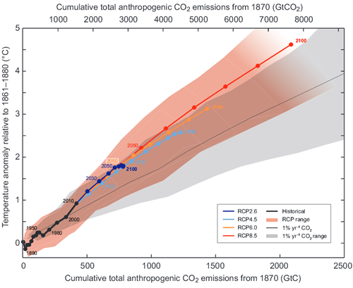
Figure 1: Increase of the mean Earth’s surface temperature as a function of the cumulative global CO2 emissions. Mean values calculated from multiple simulations using several carbon cycle models are shown until year 2100 for each RCP (color lines). Circles mark decadal means and for clarity selected decadal means were labeled with appropriate color matching text (e.g., 2050 indicates the decade 2040-2049). Black line denotes model results over the historical period (1860-2010). Shaded areas illustrate range of model results for various RCP scenarios. Black narrow line and grey shaded area show, respectively, the mean and the range of simulation results using many models CMIP5 assuming CO2 concentration growth of 1% per year. For a given value of cumulative CO2 emissions, simulations assuming 1% yearly concentration growth show smaller temperature increase than simulations corresponding to RCP, which include other forcings besides CO2. Temperature change is relative to the base period 1861-1881. Decadal averages are connected by straight lines. Source: 5th IPCC report.
The graph shows that the temperature increases almost linearly with the growth of cumulative emissions, and in case of “business as usual” scenario (red line RCP8.5) the temperature increase actually accelerates from decade to decade (as seen from the growing distance between circles marking subsequent decades). How can this observation be consistent with the logarithmic dependence between temperature increase and atmospheric CO2 concentration?
Let’s summarize several basic facts, which we will then use to reproduce Figure 1:
- Not all CO2 emissions are accumulating in the atmosphere – only about 45% of our emissions end up in the atmosphere.
- For each ppm increase of CO2 concentration the atmosphere must absorb 2.12 GtC.
- The relationship between atmospheric CO2 concentration and the corresponding increase in radiative forcing is given (3rd Report IPCC – TAR, table 6.2) by the logarithmic formula: RF = 5.35·ln (C/C0), where RF denotes radiative forcing in W/m2, C is CO2 concentration in parts per million (ppm), C0 is a reference concentration (usually the latter is 280 ppm – the concentration before the industrial revolution).
- Doubling the CO2 concentration (which is equivalent to 3.7 W/m2 increase in radiative forcing) causes temperature increase of 3°C.
Table 1 contains results of simple calculations based on observations listed above. For example, if we assume that from the beginning of the industrial era the cumulative emissions were 500 GtC (equivalent to 1833 bn tons CO2), then the atmosphere absorbed 45% of the emitted CO2, or 225 GtC. As a result atmospheric CO2 concentration has increased by 225/2.12=106 ppm, reaching level of 386 ppm, which, in turn, increases the radiative forcing by 5.35·ln (386/280) = 1.72 [W/m2]. The expected (equilibrium) temperature rise will therefore be 3·1.72/3.7=1.39 [°C].
|
Cumulative emissions |
Left in the atmosphere [GtC] |
CO2 concentration [ppm] |
Radiative forcing RF |
Equilibrium |
| 0 | 0 | 280 | 0.00 | 0.00 |
| 500 | 225 | 386 | 1.72 | 1.39 |
| 1000 | 450 | 492 | 3.02 | 2.44 |
| 1500 | 675 | 598 | 4.06 | 3.29 |
| 2000 | 900 | 705 | 4.94 | 3.99 |
| 2500 | 1125 | 811 | 5.69 | 4.60 |
Table 1. Relationship between cumulative emissions and temperature anomaly. NOTE: our model (and Figure 1) considers only carbon dioxide emissions and does not include the effects of other greenhouse gases or the cooling effect of sulfuric aerosols (these two contributions are approximately cancelling each other).
The accuracy of our model is quite good (blue line in Figure 2).
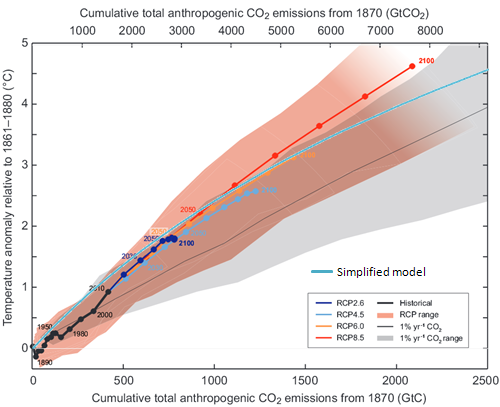
Figure 2. Results of our simple model calculations (light blue line) were added to data from Figure 1. MS Excel is available here.
Of course, such a model is very simplified. It assumes a constant airborne fraction (45%) of CO2 staying in the atmosphere. If emissions grew very fast, land and oceans sinks would be overwhelmed and would not keep pace absorbing our emissions, effectively causing larger portion of CO2 remaining in the atmosphere. According to Jones et. al., 2013, airborne fraction in RCP8.5 scenario for years 2006-2100 will go up to 69% (though uncertainity is quite large). Rising airborne fraction for huge emissions will straighten the curve. We also used the equilibrium temperature, while the real one will be somewhat smaller due to thermal inertia of the climate system.
If we include this in our model, assuming airborne fraction rising linearly from 45% (for 500 GtC of cumulative emissions) to 66% (for 2000 GtC) and display temperature anomaly as 80% of equilibrium temperature, we will get this:
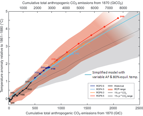
Figure 3. Results of our simple model calculations (light blue line) with variable airborne fraction and observed temperature as 80% of equilibrium temperature were added to data from Figure 1. MS Excel is available here.
We have reasonably well reproduced approximately linear relationship between cumulative emissions and the temperature anomaly, equivalent to about 1°C increase for each 500 GtC of emissions.
Exactly how quickly the temperature will rise will depend on the actual emissions rate.
Exponential growth of CO2 emissions
Historical carbon dioxide emissions can be approximated using exponential function, i.e. one that grows by a constant factor every year. That means continually increasing growth rate. In Figure 4 an exponential function growing at a rate of 2.8% yearly was superimposed on the graph of historical CO2 emissions.
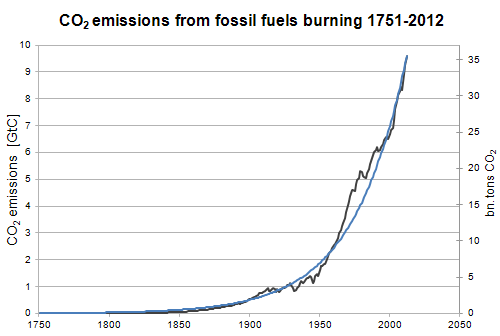
Figure 4. Growth of carbon dioxide emissions from burning fossil fuels during the period 1751-2012 (black line); source: CDIAC. Blue line represents exponential function growing at a rate of 2.8% per year (i.e. doubling every 25 years).
Such rate of growth means doubling the amount of CO2 emissions every 25 years. After 50, 75 and 100 years emissions become respectively 4 times, 8 times and 16 times larger. During the last 25 years we have emitted as much carbon dioxide from fossil fuels burning as from the beginning of the industrial revolution to the 1980s. More precisely, during 27 years between 1986 and 2012 we have emitted more CO2 than from 1751 to 1985 (CDIAC). Continuation of this trend would mean that between year 2010 and 2050 emissions would triple to a level of 100 bn tons of CO2 per year.
If the rate of emissions growth continues unchanged, in each subsequent decade we will dispose into the atmosphere ever increasing amounts of carbon dioxide, moving us ever faster to the right and upwards on the graph in Figure 1.
If we insist on burning everything we can, we will fulfill the RCP8.5 emissions scenario (or more).
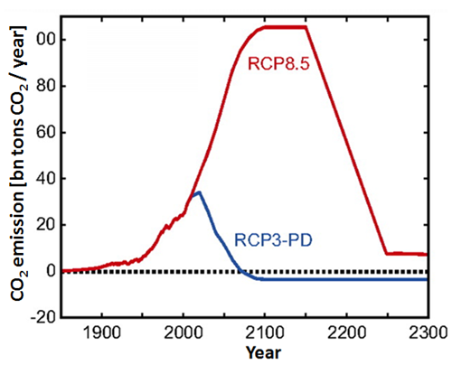
Figure 5. CO2 emissions according to two scenarios – burning all available fossil fuels (RCP 8.5) and one aiming at limiting temperature anomaly to below 2°C (RSP3-PD). In the extremely optimistic scenario RCP3-PD emissions are quickly reduced and in the middle of the XXI century fall below zero, which would mean enormous societal effort (during the lifetime of our children) of sequestration and removal from the carbon cycle of the CO2 emitted by our generation. Meinshausen et.al., 2011.
Emissions level as large as in the RCP8.5 scenario will introduce enough carbon into the carbon cycle to increase the Earth’s temperature by year 2100 by more than 4°C from the pre-industrial level (we can readily conclude this from Figure 1). Of course the temperature rise will not stop on 31 December 2100. If we assume that RCP8.5 emissions scenario continues into the next century, both axes of Figure 1 would have to be doubled in length. Simulations for this scenario (Meinshausen et.al., 2011) predict temperature anomaly by year 2200 of almost 8°C.
The future world
If we don’t change anything in our economic model (i.e. we will continue the ‘business-as-usual’ scenario), we may expect exponential growth of emissions and accelerated warming rate – in spite of “merely logarithmic” (as ‘skeptics’ emphasize) relationship between the CO2 concentration and the temperature anomaly.
Looking at Figure 1 we can immediately conclude, that if we seriously want to limit temperature anomaly to less than 2°C, we must keep the cumulative emissions below 1,000 GtC (3,666 bn tons CO2).
Marcin Popkiewicz, NaukaoKlimacie.pl; translation: Irek Zawadzki


 Arguments


I would argue that the calculations in this article are not convincing, because Figure 3 represents the dynamic response rather than hypothetical equilibrium T, assuming constant remaining atmospheric CO2 fraction. These are two different entities and the entity calculated in the article is unrealistic. It's only by coincidence, that equilibrium T curve as calculated above closely matches the IPCC dynamic temp curve in response to their scenarios.
The recent relevant literature for example Allen et al 2009, (on which the Figure 3 is based) conclude that the peak dT response to CO2 emissions (rather than equilibrium dT this article calculates) depends on the cumulative emissions but does not depend on the rate of emissions. In other words, if we burn our fossil fuels fast (e.g. RCP8.5 and stop burning abruptly due to FF limit/civilisation collapse), we reach the same maximum temperature as if we blissfuly burned FF slower (say RCP6) buf longer. The only difference is that Tmax comes earlier.
In climate change mitigaion, peak dT response is a better measure than equilibrium dT: e.g. in icesheet stability considerations.
As Allen et al have shown in their sumulations, within the range of possible antropogenic CO2 slug (1-5exagram C), the dT response is indeed linear. The reason of such response is the fact that dT signal lags the dCO2 signal due to ocean thermal inertia (resulting in delayed warming), while the remaining fraction of the original dCO2 in the atmosphere at the later time drops over time (due to ocean CO2 uptake). It turns out those two dynamic processes about cancel each other, resulting in almost linear dependence of peak dT and the emission slug. And that explanation is the key outcome, alowing a simplified measure of cumulative CO2 emissions as the only restriction is climate change mitigations.
Download the excel data and view the chart...that's not a linear relationship. The graph looks to me like a snapshot of a logarithmic curve.
I'm also confused about the Cumulative emissions: how do we know how much CO2 man's activities added to the total, and how much was due to natural sources, like volcanic activity, respiration, or organic decomposition? Why is it being expressed as a cumulative figure, when we know CO2 is absorbed by some things (like plants) and can be separated into its constituent components by natural energy releases at ambient temperatures...like a lightning storm on a warm evening.
Also, the emissions are expressed in GtC...Gigatonnes of Carbon. Don't we weight things using an independent standard...like Newtons, Grams...or Pounds? The GtC scale implies that we're only interested in the carbon...which is only part of the CO2 molecule and only 1 of 2 components (one of C & one of O2) and it’s not the heaviest of them. Oxygen is 25% heavier than Carbon...and there are two oxygen atoms per CO2 molecule. Of any amount of CO2, the portion of carbon would be 27.2% of the total...more than a quarter, less than a third. Is the graph saying that the temperature rise between freezing and 5 C (41 F) is the result of accumulating 9191 Gigatonnes of CO2? Has there ever been that much CO2 in the atmosphere at once? Ever?
[TD] For the airtight evidence that humans are responsible for 100% of the recent rise of the CO2 level in the atmosphere, see the post How Do Human CO2 Emissions Compare to Natural Emissions? There are multiple lines of evidence, but all you really need is the one that relies only on algebra.
Answering from here. This seems a better place for comment. See also article here. First, lets be clear about what is logarithmic. Doubling the concentration of CO2 from pre-industrial will increase the surface irradiation by ~4W/m2. To get another 4W/m2 of irradition, then you would have increase atmospheric concentration of CO2 to over 800ppm.
Note that is the relation between CO2 concentration and increased surface irradiation that is logarithmic - not the relationship between CO2 and temperature. Confusion of this results in a lot of strawman-arguments.
The relationship between CO2 and temperarure is much more complicated because of the various feedbacks that cut in. By itself, doubling CO2 would only raise temperature 1.1C but you cannot raise temperature without increasing the water vapour (a powerful greenhouse gas) in the atmosphere and melting ice (reducing albedo). Feedbacks work at very different timescales. Over a scale of hundreds to millenia, rising temperatures will cut in natural CO2 feedbacks (warm oceans cant hold as much dissolved CO2 and melting permafrost and clathrates release CO2 and methane). This is problem of climate sensitivity and it remains a tough problem to nail down.
Why the log dependence of irradiation on concentration. Short answer is that falls out of radiative transfer equations. For longer answer, try this paper.
Further to scaddenp's comment...the science behind the log relationship between CO2 concentration and rediative forcing can be found in Myhre et al 1998. There must be earlier papers on this but I'm not sure what they are...the refs in that paper would probably help with that.
Here are a few more helpful links:
Science of Doom: CO2: An Insignificant Trace Gas - Part Seven
RealClimate: The CO2 Problem in 6 Easy Steps and Part II of A Saturated Gassy Argument: What Angstrom didn't Know.
Since the first 20ppm of CO2 produces 50% of its GHG effect, the next doubling to 800 ppm will in crease its GHG effect by less than 2%, overwhelmed, most likely, by the other eight forcings.
There are reasons to look for alternative sources of energy. There are good reasons to clean up our environment (and our bedrooms). Plastics in the oceans and rivers should now be our main concern. And it isn't! CO2 is not a pollutant.
Climate change is a given, not a problem. CO2 mitigation is a problem, not a solution.
Jimmww @5 , the global warming effect of CO2 is not a plain logarithmic effect (also note Scaddenp's comment @ #3 above). And thus your assertion is well off-target.
Why do you say climate change "is a given" ? Taken by itself, that comment doesn't actually make sense. To make some sense of it, you really need to explain yourself, in considerable detail. Your own slogans are not sufficient.