DIY climate science: The Instrumental Temperature Record
Posted on 6 December 2012 by Kevin C
- Anyone can reproduce the instrumental temperature record for themselves, either by using existing software or by writing their own.
- A new browser-based tool is provided for this purpose.
- Many recent claims concerning climate change can be tested using this software.
The motto of the UK's Royal Society is "Nullius in verba", often translated as "Take nobody's word for it" with the implication that scientific views must be based in evidence, not authority. In this spirit, one way to test the claims of climate science is to do it yourself (DIY). There are only three scientific questions which need to be answered to determine whether climate change is a real issue:
- Is it warming?
- Why is it warming?
- What will happen in future?
The rest is window dressing. The first two questions can be addressed using the instrumental temperature record. The in situ record (based on thermometer readings) provides observations of air temperature over land and sea surface temperature which can be used to reconstruct a temperature record for much of the Earth's surface back to the 19th century. This gives a direct indication of whether the Earth is warming.
The question of why the Earth is warming may also be addressed. Warming can arise from any combination of variations in solar irradiance, albedo, and the greenhouse effect. Greenhouse-induced warming has a number of 'fingerprints' which distinguish it from the other causes, primarily stratospheric cooling (which can't be observed from the surface temperature record) but also several others (which can): The poles warming faster than the tropics, winters warming faster than summers, and nights warming faster than days (although the latter is confounded by aerosol effects).
Data can be obtained from a number of sources, including the Global Historical Climatology Network (GHCN), the Climatic Research Unit (CRU), Berkeley Earth Surface Temperature (BEST) and the International Surface Temperature Initiative (ISTI) for land temperature datasets, and the International Comprehensive Ocean-Atmosphere Data Set (ICOADS) for sea surface temperatures which is turned into geographical records including HadSST2/3, ERSST, and OISST.
Calculating a temperature record from this source data is not a very demanding task, and has been undertaken by many amateurs including Caerbannog, Nick Stokes, Steve Mosher, Zeke Hausfather, Nick Barnes and others, as well as the 'official' records from Hadley/CRU, NASA, NCDC and BEST. Calculating a record for yourself gives greater insight into the data quality, coverage and possible sources of bias. However not everyone is a programmer, so I have created a version of the calculation which can be performed in some recent web browsers (tested in Chrome 17+, Firefox 15+, Safari 6).
Rather than designing the calculation to give what I consider to be the best estimate of global surface temperature anomaly (like for example TempLS), I have made the calculation as flexible as possible so that you can experiment with different approaches. You can choose from different datasets for land and sea surface temperatures and change calculation options stepwise to switch between a HadCRUT-like and GISTEMP-like calculation. Geographical coverage is plotted along with every temperature plot, and the results can be filtered by season or latitude.
With this software you can test for yourself claims about the robustness of the data, impact of coverage, data adjustments, urbanisation, 15 year trends and greenhouse warming fingerprints. You can also add it to your own website (subject to the standard Skeptical Science license conditions), and use it as a basis for developing your own software.
Getting Started
The simplest calculation you can do is to reproduce the CRUTEM land temperature record. You will need a modern browser with good Javascript support (Firefox 15+, Chrome 17+ and Safari 6 work, as may some earlier versions, but not Internet Explorer). Launch the tool using the button below.
First you need to download the CRU station data using the first link on the page. Next uncompress the data (use software such as 7z on Windows or built-in tools on Mac or Linux).
Now scroll down and click the 'Browse' button next to 'Land station data'. Select the temperature data file that you just extracted.
Finally, click 'Calculate'. The calculation will take a few seconds, then you will be shown the results. Controls further down the page modify the display and allow data to be saved or compared. There are a number of controls which determine the calculation to be performed; these are described in the next section.
Documentation
Input data:
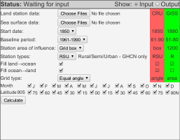
To generate a temperature record you need data. You may use land-based weather station data and/or ocean based sea surface temperature (SST) data. To get a global index you will need both. The data files are large and need to be downloaded to your computer from the data provider before you perform a temperature reconstruction.
- Land station data: Click to launch a file selector to select the land station data from your local disk. The station data needs to be in CRU3/4 format (e.g. station_data.txt) or GHCN format (ghcnm.tavg.*.qca.inv and .dat). The GHCN data is contained in two files - the inventory file (.inv) and data file (.dat) - select both of these simultaneously in the file selector (shift-click with the mouse).
Normally the GHCN average temperature ('tavg') data is used, however you can also use minimum ('tmin') or maximum ('tmax') data to obtain a record of daytime high or night-time low temperatures. Similarly you can use either the adjusted (qca) data, or the unadjusted (qcu) data.
- Ocean station data: Click to launch a file selector to select the ocean station data from your local disk. The data needs to be in HadSST format - either HadSST2 or HadSST3.
Controls:
There are a range of controls you can use to perform different calculations. Some of these allow you to select between HadCRUT-like or GISTEMP-like methods, although in practice the station area of influence is the one which makes most of the difference. The controls are as follows:
 Start date: The year in which you wish your reconstruction to start.
- Baseline period: The period over which stations will be aligned using the common anomaly method (CAM) to avoid bias due to the appearance and disappearance of stations. This should be a period when lots of records are available. HadCRUT uses 1961-1990, and GISTEMP 1951-1980.
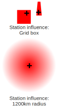
- Station area of influence: This is the most important option for choosing between a HadCRUT-like and GISTEMP-like calculation. In the HadCRUT method, a station only provides data for a single map cell, where map cells are 5°x5° and thus get narrower at higher latitudes. In the GISTEMP method, a station influences cells within a 1200km radius of the station, although nearer cells are influenced more strongly. Selecting 1200km radius will produce near-global coverage over recent decades, whereas the grid box option will give little or no coverage of the poles.
- Station types: If you are using GHCN weather station data you can filter the stations by type to include or omit Rural, Semi-rural, or Urban stations in any combination. Selecting rural stations only will address the urban heat island effect, however it will also reduce coverage and therefore increase coverage bias. A good compromise is to use rural stations only in combination with the 1200km station area of influence, thus limiting both sources of bias.
- Fill land→ocean, Fill ocean→land: These allow land temperatures to be used to provide values for empty ocean cells and vice versa. When station area of influence is set to 'grid box', coastal cells with either a land or ocean measurement are treated as having both. With the 1200km area of influence option, land temperatures can be extrapolated a long way over ocean and vice-versa. In practice this means that the Arctic can be reconstructed from surrounding land stations. (Since the Arctic is covered with ice and snow for most of the year this is not unreasonable.)
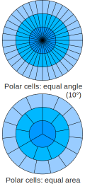 Grid type: HadCRUT uses a 5°x5° grid whose cells become narrower at higher latitudes; this means that to achieve the same coverage at high latitudes requires more densely distributed stations than at low latitudes. A more reasonable approach (used by GISTEMP and TempLS) is to reduce the number of cells at higher latitudes so that every cell covers roughly the same area. This somewhat mitigates the problem of coverage at high latitude when using grid box coverage. When using the 1200km option, the grid type is largely irrelevant.
- Months: Filtering for specific months allows calculation of seasonal temperatures for a given hemisphere. This enables you to test whether winters are warming faster or slower than summers.
- Latitudes: Filtering for specific latitude bands allows hemispheres to be selected, for example to allow the winter versus summer comparison described above. It also allows you to compare warming in different latitude bands, to test whether the poles are warming faster than the equator.
When you have set the controls as desired, click ‘Calculate’. The calculation will take a few seconds to minutes, depending on the data and options selected. The progress of the calculation is reported in the status bar above the controls.
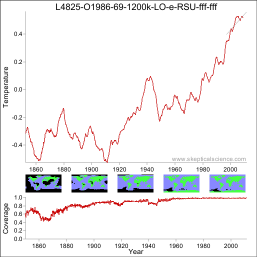
When the calculation has completed, the results will be displayed in the form of a temperature graph and a coverage graph.
The graphical display
When a calculation completes the results will be presented graphically. You can switch between the input and output displays using the buttons at the right of the status bar.
 By default the temperature series is shown as a 60 month moving average - this period may be adjusted. Global temperatures are displayed by default, however land and ocean temperatures may also be shown.
Below the temperature graph there are 5 small maps showing average data coverage over quintiles of the time range.
At the bottom is a plot of coverage with time. When land and ocean graphs are enabled this will also show land and ocean coverage as a fraction of the total land or ocean area.
Graph controls
The graph controls allow you to control some elements of data presentation which do not require a new calculation.

You change the moving average period, display land and ocean temperatures in addition to the global mean, and calculate a trend for part of the period. To add a trend to the graph, enter start and end dates into the two boxes. These are given as fractional years, thus for example to include all the data to the end of 2012, you would enter 2013 in the 'to' box.
To save a graph left-click on it. This will open a new browser window showing just the graph. Right-click this copy and select Save-as. (Firefox allows the graph to be saved directly).
Experiment log
The experiment log shows up to five previous experiments (from the current session only). Each experiment is given a title which gives a (cryptic) description of the experiment.
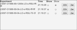
You can select which experiment is shown in the graph window using the first column of radio buttons. A second column of radio buttons allows a second set of data to be superimposed in a lighter color.
The ‘CSV’ buttons allow a tab delimited spreadsheet (.csv) file to be downloaded containing the results of a calculation. The columns are year, month, fractional year, global temperature, land temperature, ocean temperature, global coverage, land coverage, ocean coverage. You can save this file or open it in a spreadsheet program.
The 'Del' buttons allow you to delete failed experiments to make space for more results.
What can you do with it?
There are many obvious experiments you can perform with this software, only some of which I have tried. Here are some suggestions, but you can probably come up with more.
- Check if the official temperature records are realistic.
- Check how well the record produced by this software matches the official record for the appropriate set of options. (I have not tried this, but I have suggested the appropriate options to approximate the HadCRUT or GISTEMP calculations.)
- Find out to what extent the differences between the official records is determined by their source data or their methods. Try applying the GISTEMP method to the Hadley/CRU data, or the CRU method to the GHCN data.
- Test whether the poles are warming faster than the equator. Run two experiments with different settings of the latitude controls and compare the results.
- Test whether winters are warming faster than summers. Select a hemisphere using the latitude controls, then run two experiments with different sets of months and compare the results.
- Estimate the impact of the urban heat island effect: Using the GHCN data run calculations using stations of type R,S,U or R only. Note that using rural stations only will impact coverage, which will also change the results. To avoid this use the 1200km area of influence option.
- Determine the impact of the GHCN adjustments: Run two calculations to compare the adjusted (qca) versus unadjusted (qcu) data. The magnitude of the difference is of course strongly influenced by whether you include ocean data as well.
- Compare the results using various settings with Caerbannog's new software which will run in a virtual machine.
Advanced calculations
There are some more advanced calculations which may be performed by using the GHCN data and editing the inventory file to control which stations are used in the calculation. Any station which is missing from the inventory file will not be used. Therefore by creating a copy of the inventory file with a reduced station list you can examine the effects of using different subsets of stations. Manipulating the inventory file by hand is time consuming, so I have provided useful commands which can be used to perform these manipulations automatically from a Mac or Linux command-line.
- Reducing the number of stations.
An important question is whether there is sufficient data to reliably determine a temperature record. This is easily tested by reducing the number of stations and testing whether the results are affected.
Make a copy of the file containing the station inventory (either qcu.inv or station-data.txt). This copy can be edited to select specific stations. For the GHCN data, simply delete the line for any station you wish to omit. For the CRU data, set the latitude of the station (second field, characters 7-10) to -999.
To calculate a record with just 10% of the data you can take every 10th station. You can select multiple subsets to compare. On Mac/Linux:
awk "NR%10==0" qcu-XXXX.inv > qcu-0of10.invThen rerun the calculation using each inventory file in turn and compare the results.
awk "NR%10==1" qcu-XXXX.inv > qcu-1of10.inv
awk "NR%10==2" qcu-XXXX.inv > qcu-2of10.inv - Filter GHCN stations based on the urban night-light field:
grep 'A$' qcu.inv > qcu-rural.inv
- Calculating records for different countries.
For GHCN create a new .inv file using just the stations starting with the relevant country code. e.g. to select only US weather stations use:
grep '^425' qcu-XXXX.inv > qcu-usa.inv
Note that the program cannot mask the results to cover the precise borders of an individual country, so the results will be approximate.
Browser compatibility
The following table indicates browsers which are known to work with the software:
| Chrome | Firefox | Safari | Opera | Explorer | |
| Not working | ? | ? | ? | 1-12 | 1-8 |
| Partially working | ? | 10 | ? | - | ? |
| Fully working | 17-20 | 15-16 | 6 | - | ? |
What now?
Go and do some science. Please post interesting results, bugs and browser compatibility notes in the comments below (although please be clear about the settings you are using). You can also use the tool to test claims you encounter elsewhere concerning the instrumental record. You probably don't want to cite the results in a peer-reviewed publication, but they may be useful for preliminary trials.


 Arguments


Note: The CSV download button is currently not working. As far as I am aware everything else is fine. A fix is on its way to John Cook. I'll update this comment once it's fixed.Now fixed, thanks Doug!- The page title of the calculator page is "Skeptical Science Email Subscription".
- I think the sentence "Ocean station data: Click to launch a file selector to select the land station data ..." should read "Ocean station data: Click to launch a file selector to select the ocean station data ..."
Otherwise, very impressive. As a Linux/Firefox user, I shall have fun playing with this. Thanks for all the work, Kevin C.