Climate Science Glossary

Term Lookup

Enter a term in the search box to find its definition.

Settings

Use the controls in the far right panel to increase or decrease the number of terms automatically displayed (or to completely turn that feature off).

Term Lookup

Settings


All IPCC definitions taken from Climate Change 2007: The Physical Science Basis. Working Group I Contribution to the Fourth Assessment Report of the Intergovernmental Panel on Climate Change, Annex I, Glossary, pp. 941-954. Cambridge University Press.

Home Arguments Software Resources Comments The Consensus Project Translations About Support

Bluesky Facebook LinkedIn Mastodon MeWe

Twitter YouTube RSS Posts RSS Comments Email Subscribe


Climate's changed before
It's the sun
It's not bad
There is no consensus
It's cooling
Models are unreliable
Temp record is unreliable
Animals and plants can adapt
It hasn't warmed since 1998
Antarctica is gaining ice
View All Arguments...


Username
Password
New? Register here
Forgot your password?

Latest Posts

Archives

A detailed look at Hansen's 1988 projections

Posted on 20 September 2010 by dana1981

Hansen et al. (1988) used a global climate model to simulate the impact of variations in atmospheric greenhouse gases and aerosols on the global climate.  Unable to predict future human greenhouse gas emissions or model every single possibility, Hansen chose 3 scenarios to model.  Scenario A assumed continued exponential greenhouse gas growth.  Scenario B assumed a reduced linear rate of growth, and Scenario C assumed a rapid decline in greenhouse gas emissions around the year 2000.

Misrepresentations of Hansen's Projections

The 'Hansen was wrong' myth originated from testimony by scientist Pat Michaels before US House of Representatives in which he claimed "Ground-based temperatures from the IPCC show a rise of 0.11°C, or more than four times less than Hansen predicted....The forecast made in 1988 was an astounding failure." 

This is an astonishingly false statement to make, particularly before the US Congress.  It was also reproduced in Michael Crichton's science fiction novel State of Fear, which featured a scientist claiming that Hansen's 1988 projections were "overestimated by 300 percent." 

Compare the figure Michaels produced to make this claim (Figure 1) to the corresponding figure taken directly out of Hansen's 1988 study (Figure 2).
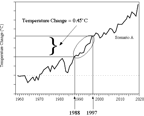
 

Figure 1: Pat Michaels' presentation of Hansen's projections before US Congress
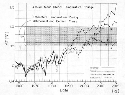
 

Figure 2: Projected global surface air temperature changes in Scenarios A, B, and C (Hansen 1988)

Notice that Michaels erased Hansen's Scenarios B and C despite the fact that as discussed above, Scenario A assumed continued exponential greenhouse gas growth, which did not occur.  In other words, to support the claim that Hansen's projections were "an astounding failure," Michaels only showed the projection which was based on the emissions scenario which was furthest from reality. 

Gavin Schmidt provides a comparison between all three scenarios and actual global surface temperature changes in Figure 3.
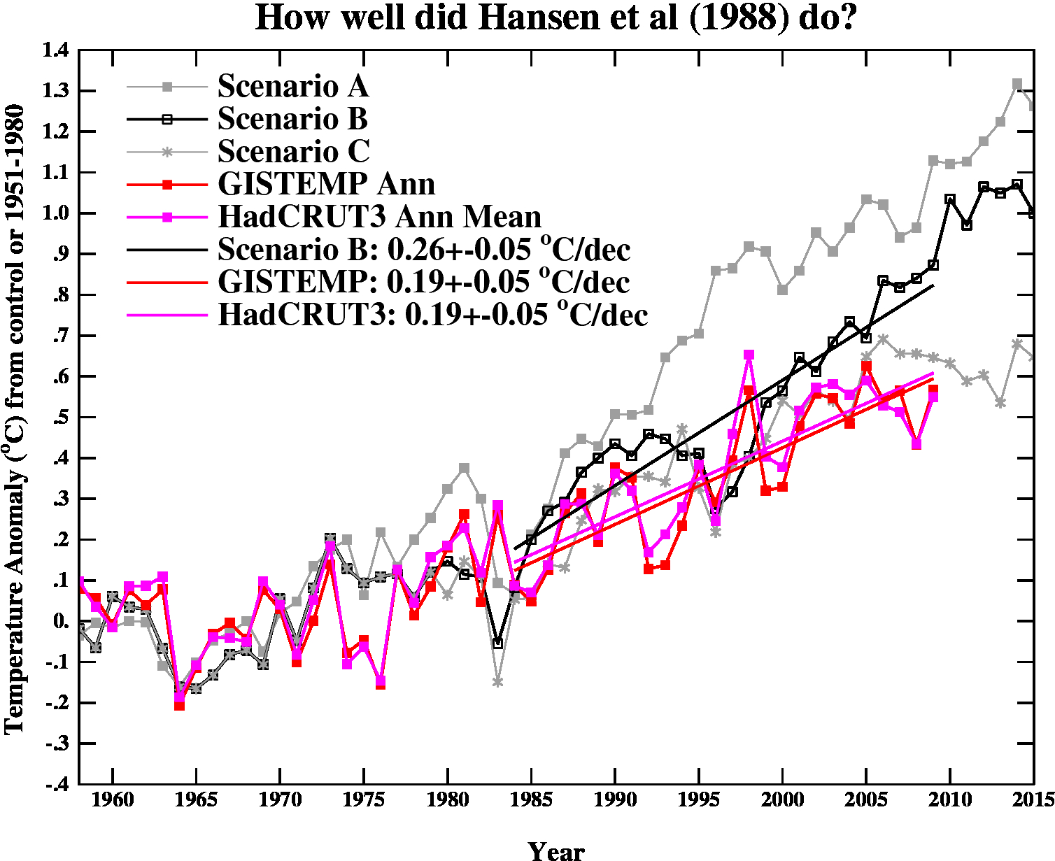
 

Figure 3: Hansen's projected vs. observed global temperature changes (Schmidt 2009)

As you can see, Hansen's projections showed slightly more warming than reality, but clearly they were neither off by a factor of 4, nor were they "an astounding failure" by any reasonably honest assessment.  Yet a common reaction to Hansen's 1988 projections is "he overestimated the rate of warming, therefore Hansen was wrong."   In fact, when skeptical climate scientist John Christy blogged about Hansen's 1988 study, his entire conclusion was "The result suggests the old NASA GCM was considerably more sensitive to GHGs than is the real atmosphere."  Christy didn't even bother to examine why the global climate model was too sensitive or what that tells us.  If the model was too sensitive, then what was its climate sensitivity?

This is obviously an oversimplified conclusion, and it's important to examine why Hansen's projections didn't match up with the actual surface temperature change.  That's what we'll do here.

Hansen's Assumptions

Greenhouse Gas Changes and Radiative Forcing

Hansen's Scenario B has been the closest to the actual greenhouse gas emissions changes.  Scenario B assumes that the rate of increasing atmospheric CO2 and methane increase by 1.5% per year in the 1980s, 1% per year in the 1990s, 0.5% per year in the 2000s, and flattens out (at a 1.9 ppmv per year increase for CO2) in the 2010s.  The rate of increase of CCl3F and CCl2F2 increase by 3% in the '80s, 2% in the '90s, 1% in the '00s, and flatten out in the 2010s. 

Gavin Schmidt helpfully provides the annual atmospheric concentration of these and other compounds in Hansen's Scenarios.  The projected concentrations in 1984 and 2010 in Scenario B (in parts per million or billion by volume [ppmv and ppbv]) are shown in Table 1.

Table 1: Scenario B greenhouse gas (GHG) concentration in 1984, as projected by Hansen's Scenario B in 2010, and actual concentration in 2010


GHG 

1984 

Scen. B 2010 

 Actual 2010

CO2  344 ppmv  389 ppmv  392 ppmv
N2O  304 ppbv  329 ppbv  323 ppbv
CH4  1750 ppbv  2220 ppbv  1788 ppbv
CCl3F  0.22 ppbv  0.54 ppbv  0.24 ppbv
CCl2F2  .038 ppbv  0.94 ppbv  0.54 ppbv


We can then calculate the radiative forcings for these greenhouse gas concentration changes, based on the formulas from Myhre et al. (1998).

dF(CO2) = 5.35*ln(389.1/343.8) = 0.662 W/m2

dF(N2O) =  0.12*(N - N0) - (f(M0,N) - f(M0,N0))

= 0.12*(329 - 304) - 0.47*(ln[1+2.01x10⁻⁵ (1750*329)0.75+5.31x10⁻¹⁵ 1750(1750*329)1.52]-ln[1+2.01x10⁻⁵ (1750*304)0.75+5.31x10⁻¹⁵ 1750(1750*304)1.52]) = 0.022 W/m2

dF(CH4) =0.036*(M - M0) - (f(M,N0) - f(M0,N0))

= 0.036*(2220 - 1750) - 0.47*(ln[1+2.01x10⁻⁵ (2220*304)0.75+5.31x10⁻¹⁵ 2220(2220*304)1.52]-ln[1+2.01x10⁻⁵ (1750*304)0.75+5.31x10⁻¹⁵ 1750(1750*304)1.52]) = 0.16 W/m2

dF(CCl3F) = 0.25*(0.541-0.221) = 0.080 W/m2

dF(CCl2F2) = 0.32*(0.937-0.378) =  0.18 W/m2

Total Scenario B greenhouse gas radiative forcing from 1984 to 2010 = 1.1 W/m2

The actual greenhouse gas forcing from 1984 to 2010 was approximately 1.06 W/m2 (NASA GISS).  Thus the greenhouse gas radiative forcing in Scenario B was too high by about 5%.

Climate Sensitivity

Climate sensitivity describes how sensitive the global climate is to a change in the amount of energy reaching the Earth's surface and lower atmosphere (a.k.a. a radiative forcing).  Hansen's climate model had a global mean surface air equilibrium sensitivity of 4.2°C warming for a doubling of atmospheric CO2 [2xCO2].  The relationship between a change in global surface temperature (dT), climate sensitivity (λ), and radiative forcing (dF), is

dT = λ*dF

Knowing that the actual radiative forcing was slightly lower than Hansen's Scenario B, and knowing the subsequent global surface temperature change, we can estimate what the actual climate sensitivity value would have to be for Hansen's climate model to accurately project the average temperature change.

Actual Climate Sensitivity

One tricky aspect of Hansen's study is that he references "global surface air temperature."  The question is, which is a better estimate for this; the met station index (which does not cover a lot of the oceans), or the land-ocean index (which uses satellite ocean temperature changes in addition to the met stations)?  According to NASA GISS, the former shows a 0.19°C per decade global warming trend, while the latter shows a 0.21°C per decade warming trend.  Hansen et al. (2006) – which evaluates Hansen 1988 – uses both and suggests the true answer lies in between.  So we'll assume that the global surface air temperature trend since 1984 has been one of 0.20°C per decade warming.

Given that the Scenario B radiative forcing was too high by about 5% and its projected surface air warming rate was 0.26°C per decade, we can then make a rough estimate regarding what its climate sensitivity for 2xCO2 should have been:

λ = dT/dF = (4.2°C * [0.20/0.26])/0.95 = 3.4°C warming for 2xCO2

In other words, the reason Hansen's global temperature projections were too high was primarily because his climate model had a climate sensitivity that was too high.  Had the sensitivity been 3.4°C for a 2xCO2, and had Hansen decreased the radiative forcing in Scenario B slightly, he would have correctly projected the ensuing global surface air temperature increase.

The argument "Hansen's projections were too high" is thus not an argument against anthropogenic global warming or the accuracy of climate models, but rather an argument against climate sensitivity being as high as 4.2°C for 2xCO2, but it's also an argument for climate sensitivity being around 3.4°C for 2xCO2.  This is within the range of climate sensitivity values in the IPCC report, and is even a bit above the widely accepted value of 3°C for 2xCO2.

Spatial Distribution of Warming

Hansen's study also produced a map of the projected spatial distribution of the surface air temperature change in Scenario B for the 1980s, 1990s, and 2010s.  Although the decade of the 2010s has just begun, we can compare recent global temperature maps to Hansen's maps to evaluate their accuracy.

Although the actual amount of warming (Figure 5) has been less than projected in Scenario B (Figure 4), this is due to the fact that as discussed above, we're not yet in the decade of the 2010s (which will almost certainly be warmer than the 2000s), and Hansen's climate model projected a higher rate of warming due to a high climate sensitivity.  However, as you can see, Hansen's model correctly projected amplified warming in the Arctic, as well as hot spots in northern and southern Africa, west Antarctica, more pronounced warming over the land masses of the northern hemisphere, etc.  The spatial distribution of the warming is very close to his projections.
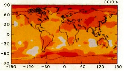
 

Figure 4: Scenario B decadal mean surface air temperature change map (Hansen 1988)
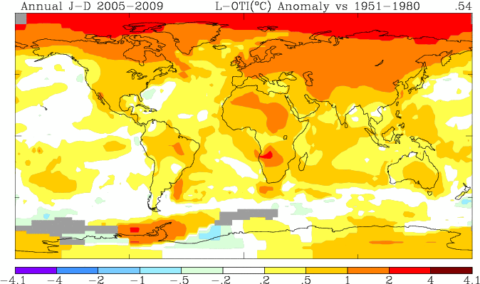
 

Figure 5: Global surface temperature anomaly in 2005-2009 as compared to 1951-1980 (NASA GISS)

Hansen's Accuracy

Had Hansen used a climate model with a climate sensitivity of approximately 3.4°C for 2xCO2 (at least in the short-term, it's likely larger in the long-term due to slow-acting feedbacks),  he would have projected the ensuing rate of global surface temperature change accurately.  Not only that, but he projected the spatial distribution of the warming with a high level of accuracy.  The take-home message should not be "Hansen was wrong therefore climate models and the anthropogenic global warming theory are wrong;" the correct conclusion is that Hansen's study is another piece of evidence that climate sensitivity is in the  IPCC stated range of 2-4.5°C for 2xCO2.

This post is the Advanced version (written by dana1981) of the skeptic argument "Hansen's 1988 prediction was wrong". After reading this, I realised Dana's rebuttal was a lot better than my original rebuttal so I asked him to rewrite the Intermediate Version. And just for the sake of thoroughness, Dana went ahead and wrote a Basic Version also. Enjoy!


0 0

Printable Version  |  Link to this page

Comments

Prev  1  2  3  Next

Comments 51 to 100 out of 128:

  1. Joe, "I would consider 23% more sensitive substantial" Dana is addressing misleading statement made by Michaels and Christy-- I have also addressed that in my post @46. Regardless, what you might consider or think is "substantial" is not necessarily indicative of what the reality is. The range given by IPCC for CS is 1.5 through 4.5 C. Hansen's original model had a CS was clearly on the high end of that range, I for one am not trying to ignore that. What I take issue is with certain people spinning that. Can I assume that you agree with what Michaels and Christy have said on this? Science advances, Hansen had the intellect, know how and guts to make a bold prediction, that all things considered, was in good agreement with what actually transpired (predicted warming of 0.26 C per decade versus observed warming almost 0.20 C per decade). I doubt that you, or I, or Michaels would venture to make such a prediction and get it even remotely correct. Anyhow, that is the nature of science. You give it you best shot, using the best tools and information at your disposal now, and then someone else comes along and improves upon your technique, or down the road you improve upon your initial work. Hansen's seminal work has served as a building block for others.
    0 0
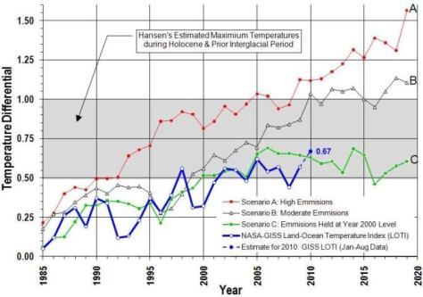
  2. #43 Albatross, you are correct that Pat Michaels misled Senate but so has Dana1981 in this post. The NASA GISS data up to August 2010 are shown in Figure 1. They are compared with Scenarios A, B and C in Hansen (2006). The blue line denotes the Land-Ocean Temperature Index (LOTI). Figure 1: Scenarios A, B and C Compared with Measured NASA GISS LOTI (after Hansen, 2006) I have used the LOTI data in Figure 1 because the GISS website states that this provides the most relaistic representation of global meam trends. It is evident from Figure 1 that the best fit for actual temperature measurements is currently the emissions-held-at-year-2000-level Scenario C. Therefore it is incorrect for Dana1981 to contend that temperaturea are currently following a trajectory slightly below Scenarion B. Nevertheless, I do agree #23 CBDunkerson that the time period is still relatively short for comparing the scenarios. Consequently I agree with Hansen (2006) that we should wait until 2015 for distinction between the scenarios and useful comparison with the real world.
    0 0
  3. Angusmac, Nice graph. You use your Fig. 1 (which is what I assume to be an accurate replication of Fig. 2 in Hansen et al. (2006)) to make the assetion that: "It is evident from Figure 1 [after Hansen. 2006] that the best fit for actual temperature measurements is currently the emissions-held-at-year-2000-level Scenario C". Let us have a look at Hansen et al. (2006). They state that: "Modeled 1988–2005 temperature changes are 0.59, 0.33, and 0.40°C, respectively, for scenarios A, B, and C. Observed temperature change is 0.32°C and 0.36°C for the land–ocean index and meteorological station analyses, respectively. Warming rates in the model are 0.35, 0.19, and 0.24°C per decade for scenarios A, B. and C, and 0.19 and 0.21°C per decade for the observational analyses." Now either Hansen et al. made a mistake and inadvertently swapped the warming rates for scenario B and C, or your claim (cited above) which is based on your Figure 1 is false. Because the warming rate for scenario B of +0.19 C is the same as the observed rate of warming in the LOTI data. You state that Now there is an important caveat here of course, the data in Hansen et al. (2006) are for a different time window considered by Schmidt (2009). I do agree that it would be helpful if the predicted rate of warming for 1984-2009 for Scenario C could be included in Fig. 3 in the post. It is evident that the time windows chosen to validate the projections yield different answers. But, even so, the claims made by Crichton and others are incorrect and misleading. Hansen et al. (2006) also conclude that: "Nevertheless, it is apparent that the first transient climate simulations (12) proved to be quite accurate, certainly not ‘‘wrong by 300%’’ (14)"
    0 0
  4. @NETDR: "The Pat Michaels analysis is a straw-man defense." I'm not sure you know what a strawman argument is. What Albatross (not CBD) said certainly wasn't a strawman; for that, he would have had to ascribe to you an opinion that wasn't yours. "Dr Hansen's model was seriously wrong but not as seriously as Pat said. So what?" There is such a thing as "a little wrong", "seriously wrong" and "completely wrong" in science. You seem to believe that it's a binary condition, i.e. one is either wrong or right. Unfortunately, reality doesn't like such absolutes. "For this we are seriously discussing tens of trillions of dollars of taxes and cap and trade ?" Careful, your bias is showing. An important fact for you to consider: if you agree with the analysis that shows Hansen was off on climate sensitivity by 0.8C for his choice of a 4.2C value, this means you *do* agree with a figure of about 3.4C for climate sensitivity. Let me put it another way: either you agree that climate sensitivity is about 3.4C, or you don't believe this critique of Hansen 1988 is accurate, and thus can't use it this particular evidence to support your affirmation that Hansen got it wrong. So, before we go any further, do you agree with the 3.4 figure for climate sensitivity? "So this article has proven he was wrong [in 88] and claimed it was a rebuttal to those that claim he was wrong. [in 88] Am I missing something ???" Yes, you are, but your use of multiple interrogation point and apparent obsession for boolean certainty in science make me wary of continuing this dialogue. @Joe Blog: "But the Q is, did Hansen 88 accurately model climate since its hindcast... the answer is no." Another, equally valid answer, would be that he answered it more accurately than others at the time. It's important to note that Hansen later acknowledged the differences, as this article does. The topic here is how contrarians have used the inaccuracy as an excuse to grossly underestimate climate sensitivity. That's the whole point of the article, unless I'm mistaken.
    0 0
  5. @Angusmap: "It is evident from Figure 1 that the best fit for actual temperature measurements is currently the emissions-held-at-year-2000-level Scenario C. Therefore it is incorrect for Dana1981 to contend that temperaturea are currently following a trajectory slightly below Scenarion B." As I understand it, the question is not whether the actual record is closer to B or C, because we know real-world emissions are closer to emmission scenario B. Thus accuracy of the model has to be gauged in relation to scenario B. Had emmissions been closer to C, then we'd be comparing the record with C, and would find Hansen 1998 had been amazingly accurate! :-) Am I getting this right?
    0 0
  6. Archiesteel @55, You just stated what I was thinking of saying, but more eloquently and succinctly than I am capable of. Earlier I suggested including the rate of warming for the 1984-2009 window for Scenario C, but in retrospect it is pointless comparing observations with Scenario C much beyond 2000 b/c the emissions (i.e., GHG forcing) for Scenario C after 2000 are not realistic. I suspect that is the reason why Schmidt and Dana did not include it in their analyses which extend almost a decade beyond 2000. Hansen et al. included Scenario C in their validation up until 2005, and that, IMHO, was probably pushing it. Anyhow, FWIW, you are getting it right :)
    0 0
  7. Archiesteel 55 RE: Strawman defense: I had never before read Pat Michaels views on the subject. Selecting his extreme views as a straw-man to do battle with is lame. They in no way reflect my views or any skeptics I know of. Reading the graph of Dr Hansen's predicted warming and the climates refusal to co-operate with him doesn't take a PhD. Anyone with the ability to do simple math can figure out how wrong he was. See my previous posts. Actual temperature was below scenario "C" which was with carbon taxes and restrictions. I don't have to have any particular view of AGW to believe that only 44 % of the predicted warming occurred between 1988 and 2009. That is a fact. Some other parameter could be wrong, the only thing we know for sure is that the answer was wrong. The rest is just speculation. By the way at that [1988 to 2009] rate of warming in 100 years turns out to be about 1 ° C which would be beneficial. My having a particular belief of climate sensitivity or use this article. is a false choice. You spin fallacy after fallacy, Who needs this article to prove what almost any high school student can compute for himself? Far from being Boolean a model which predicts so much warming that only 44 % of it occurs is broken. There is a big difference between being close and the miserable performance of his model so far. The errors compound so by 100 years from now the error will be huge. Better luck on the net model. Just don't post the results where the public can compare them with reality.
    0 0
  8. Albatross and archiesteel are correct. Apparently it would have behooved me to pull a Michaels and erase Scenarios A and C from the figure, because so many people can't get past "it looks like C!". Scenario C is irrelevant because it does not accurately reflect the actual emissions, unlike Scenario B, which is quite close. The fact that actual temps have been close to those in Scenario C doesn't matter in the least. Joe Blog nailed the problem in #44: "Im not drawing any other conclusion from this, other than Hansen had it wrong in 88." That's the problem with Joe, angusmac, NETDR, etc. The entire purpose of this rebuttal was to go beyond that grossly oversimplified and frankly useless conclusion. Of course Hansen didn't perfectly project the future warming rate. The question is why not? The answer is that his model's climate sensitivity was too high. No, Hansen's model was not perfect. Yes it was off by around 25%. But that's a useless conclusion. Climate models weren't perfect 22 years ago, what a newsflash. The useful conclusion is that this tells us that the actual climate sensitivity is in the ballpark of 3.4°C for 2xCO2, which is right in the middle of the IPCC range, and approximately the average climate sensitivity of today's climate models. Also given the fact that Hansen's model could have projected anything from rapid cooling to no change to rapid warming, being off by 25% on the warming trend really ain't that bad.
    0 0
  9. NETDR # 57 - "I don't have to have any particular view of AGW to believe that only 44 % of the predicted warming occurred between 1988 and 2009. That is a fact." No, actually it's not even remotely a fact. Generally speaking, for something to be a fact, it has to be true. The correct statement is that *77%* of the *projected* warming between 1988 and 2010 occurred. You'll never get the correct figure by cherrypicking the data points you like; you have to look at the trends (0.26°C per decade vs. 0.20°C, as discussed in the article).
    0 0
  10. Dana 59 Using 5 year averages to avoid cherry picking. The chart predicts[1988-2009] .9 °C - .25 °C = .65°C warming. Reality [1988 to 2009] is .54 - .25 = .29 °C Using GISS's own data. Predicted warming = .29/.65 = 44.6 % Where you got the 77 % I will probably never know. Dr Hansen picked this particular cherry. He should know that the climate is a negative feedback system [as defined in physics not climatology] Since it was warming in the years just before 1988 a cooling was inevitable. He should have factored that in. An overshoot like 1998 was followed by an undershoot in 1999 and 2000 it is predictable in negative feedback systems. [Climatology defines positive feedback differently than all of the other sciences.] When "the debate is over" and you know all of the answers you have to know all of the answers.
    0 0
  11. @NETDR: So, just to be clear, you *don't* agree with Michaels when he says "the forecast made in 1988 was an astounding failure." I'm just trying to establish your position here. It's kind of tricky with deniers (which you clearly are, by your approach and choice of rhetoric). "Reading the graph of Dr Hansen's predicted warming and the climates refusal to co-operate with him doesn't take a PhD." Actually - and this is the whole point of the article - the climate "sort of" cooperated with his assessment, i.e that temperatures were going to go up by a significant amount. He overestimated the final result, but got it mostly right compared to, say, someone who would have argued it was going to be cooling, or that temperatures were going to stay the same. Your absolutism fools no one, you know... "My having a particular belief of climate sensitivity or use this article. is a false choice." Of course not. It's simple logic: either you think the argument is scientifically valid, or you don't. You just want to cherry-pick the parts you like, and ignore the parts you don't. Typical. "You spin fallacy after fallacy," I certainly do not. You, on the other hand, are clearly trying to push an agenda. "Far from being Boolean a model which predicts so much warming that only 44 % of it occurs is broken." Not 44%. The error was 0.8 on 3.4, so about 1/4. Hansen got it about 75% right. But keep on ignoring the arguments presented to you, and restating the same faulty calculation. You're really gonna go far with that one.
    0 0
  12. NETDR @60, "Where you got the 77 % I will probably never know." Try this: 0.20/0.26 = .... Actually, I disagree slightly with Dana and suggest that for 1984-2009, 73% of the predicted warming was realised (0.19/0.26). But there are those error bars in the observed and predicted warming, so I should not nit pick at differences of 0.01 C when the error bars are 0.05 ;) How about, approximately 75% of the predicted warming between 1984 and 2009 was realised.
    0 0
  13. Swinging back to the original point of this article, its about misrepresentation. Claiming the temperature results from high emission scenario were Hansen's prediction and comparing that curve to actual temperatures which are actually more relevant to a different scenario is out and out dishonest. Redtrawing the graph so that those "confusing" other curves which would give a clearer picture shows this was a deliberate attempt to mislead. Hansen on the other hand is giving the results for the best climate model available at the time. He didnt CHOOSE a sensitivity of 4.2 - this is an output from the model. Are we surprised that model got it wrong considering how primitive it was? No, and we now understand why it was wrong too. We still struggle to get an accurate number for short-term (10-30 year) climate sensitivity. An imperfect model is not dishonesty.
    0 0
  14. NETDR - if you don't know where I'm getting 77% then you've read neither the article nor my comments (or can't divide 0.20 by 0.26, as Albatross illustrates). I have no idea where you're getting yours from - cherrypicking favorable data points no doubt. Albatross - I explain in the article why I use 0.20. It's the 'surface air temperature' issue and how that's defined. But using 75% is fine, I like rounding. I guess my problem here is that I'm expecting readers and commenters at Skeptical Science to think like skeptical scientists. A skeptical scientist does not say "Hansen was wrong and I don't care why." That's incredibly unscientific. It's critical to know what is responsible for scientific inaccuracies. For example, why was the UAH satellite temperature data so radically different from surface station data a decade ago? Were the satellites wrong? Were the surface stations wrong? Was somebody fudging the numbers or screwing up the analysis? No scientist would simply say "oh well the temperature data is just wrong and I don't care why." I think the problem here is clearly that "Hansen was wrong" is a much more convenient conclusion for certain biased individuals than "Hansen's results are evidence that the IPCC and today's climate models have the climate sensitivity right".
    0 0
  15. @NETDR: "Using 5 year averages to avoid cherry picking." To avoid cherry picking, use the linear trends for both Scenario B and the temp record. Using averages but arbitrarily choosing dates is still cherry-picking.
    0 0
  16. Dana @64. Mea culpa Dana. Sorry. I really need to stop multi-tasking. As you noted, you state in the post: "So we'll assume that the global surface air temperature trend since 1984 has been one of 0.20°C per decade warming."
    0 0
  17. NETDR @48 4.2-3.4=.8 /4.2 = 0.19=19% = that is how much Hansen is off from reality. You keep coming up with 44% by "eyeballing" .9 where .9 does not exist. What is the point of discussing if you don't keep your posts based in reality?
    0 0
  18. I must have got this seriously wrong. AFAIK climate sensitivity is an outcome of the climate models, not an input.
    0 0
  19. There is a very interesting phenomena at work here - not just restricted to the deniers. Hansen's 1988 graphs show 3 lines, based on 3 sets of inputs. We all (except for Michaels - but it is 2010 - I personally have no time for those that deny the world is warming)... so we easily rule out scenario "A" - neither the emissions nor the temperatures line up - so out the window it goes. Dana1981 presents the information, with technical support. I think I am accurately paraphrasing Dana1981 to say: Only scenario B is worth looking at - because that is a pretty close match to actual emissions. Scenarios A and C are provided for completeness and context, but are not germane to the discussion." Many readers (and I include myself) need at least an acknowledgement that actual temperatures are at/near/below Scenario C (or to have our noses dragged through the point that "C" doesn't matter BECAUSE the actual emissions don't match that Scenario). I know realize that the whole point is to compare Scenario B temperatures to reality, because Scenario B matches the emissions - but my first reading I was wondering why Scenario "C" - which looks like a good match (based on temperature), is irrelevant. I think this is the difference between rigorous scientific thinking, and interested bystander thinking. Anyways, it is one reason why I like this blog - thank you for making that point clear to me! Regarding my post 67 comes up with 19% because I choose 4.2 for the denominator. I think that is valid because it is Hansen's error divided by Hansen's choice - rather than Hansen's error divided by reality - mine is internally consistent. But I grant that it is pretty much semantics at this point. Finally - for anyone to look at this and be anything but amazed that someone, in 1988 - when all the theories of climate that EVENTUALLY became AGW were still in the "maybe" column and not be amazed at how prescient and accurate Hansen was, just befuddles me!
    0 0
  20. John, is there an assumption in your calculations that 100% of the temperature rise over this period is due to the forcing of human GHGs? Because the IPCC's "most" is starting to look like "all".
    0 0
  21. The other question I have is to do with scenario A, B and C. Having read the paper I'd sort of assumed that A was the "business as usual" option and the catastrophists really on this for the fearful future. Is this a wrong assumption on my part?
    0 0
  22. Posted by dana1981 on Monday, 20 September, 2010 at 11:38 AM Had Hansen used a climate model with a climate sensitivity of approximate 3.4°C for 2xCO2 (at least in the short-term, it's likely larger in the long-term due to slow-acting feedbacks), he would have projected the ensuing rate of global surface temperature change accurately. Not only that, but he projected the spatial distribution of the warming with a high level of accuracy. OK, let's have a closer look. Hansen 1988 has also predicted the decadal mean temperature change for scenario B as a function of pressure and latitude. Now, since then we have got some actual data about this temperature trend distribution. The Hadley Centre of the UK Met Office has a near real-time updated dataset called HadAT (globally gridded radiosonde temperature anomalies from 1958 to present).
    Linear trends in zonal mean temperature (K/decade) in HadAT2 1979-2009. 1000 hPa data are from HadCRUT2v subsampled to the time-varying HadAT2 500hPa availability
    The image above is explained in this publication: Internal report for DEFRA, pp. 11 HadAT: An update to 2005 and development of the dataset website Coleman, H. and Thorne, P.W. As you can clearly see, predicted and observed zonal trends have nothing to do with each other: neither high, nor low level of accuracy can be detected. Particular attention should be payed to the cooling trend in the tropical mid-troposphere (-0.5°C/century) and the severe cooling between 65S and 70S along the entire air column (down to -5°C/century). These features are absolutely lacking in Hansen's prediction, therefore the take-home message should be "Hansen's 22 year old prediction is falsified". We can talk about if anthropogenic global warming theory were wrong on which the model was based or it was a flawed implementation, but there is no question about Hansen's failure. BTW, the tropical upper tropospheric cold spot observed and documented in HadAT2 is inconsistent with surface warming according to even the most recent computational climate models. So neither Hansen nor his followers can get the sign of change right in some particularly important regions. Taking into account this wider failure, we can safely bet "climate models and the anthropogenic global warming theory are wrong", quite independent of Hansen's 1988 blunder.
    0 0
  23. Sorry Dana I didn't see you were the author. #70 is aimed at you.
    0 0
  24. @Albatross: On the one hand, I can understand why it is important to debunk all of the false charges made about the validity of forecasts made by Dr. James Hansen in 1998. On the other hand, given how far the state-of-art in climate modeling has advanced over the past two decades plus, why is the validity of forecasts made in 1998 cause for such consternation today? I’m not a scientist. I’m just trying to learn the lay of the land so to speak.
    0 0
  25. Hi Badger, Good question. The only reason I can think of is because to this day "skeptics" and those in denial about AGW keep touting Hansen's projection as "evidence" that climate models do not work at all. Or, that the projections were "wrong" then and so they will all be wrong now-- silly logic, but for those not in the know such statements are at the very least confusing and/or sow doubt, especially when not provided context or updates on the latest developments. So sadly, people like John and Dana have to spend their valuable time addressing the confusion and trying to undue the confusion. A perfect analogy for this Hansen paper is the 1998 Hockey Stick paper (MBH98), MBH98 did have some issues (like all seminal techniques it was not perfect), but he science has advanced (in part b/c of that seminal work) and technique shave been improved upon or refined, yet the contrarians to this day are still stuck 1998, or is that 1988? My suggestion to NETDR, BP and HR (and HR enough with the rhetoric already HR (e.g., "catastrophists") is to please move on.
    0 0
  26. Anne van der Bom - you are correct, and I tried to be careful in my phrasing. Hansen employed a climate model which had a climate sensitivity of 4.2°C for 2xCO2. actually thoughtfull - you got it. All Scenarios are included for completeness, but it really only makes sense to look at B. We could look at C and adjust for the differences in GHGs there too, but there's no much point, since B is closer to reality. As for the percentages, Hansen's model sensitivity was off by 19% and his temp projections were off by 23%, the difference being the 5-10% excess in Scenario B forcing as compared to actual forcing. HumanityRules - approximately 100% of the temp change since 1984 has been to GHGs. The IPCC looks at the temp change over a longer period of time, which has been partially natural. Scenario A is constantly accelerating GHG emissions, whereas B is a linear increase in emissions. Thus Scenario B is effectively business as usual. Berényi Péter - the tropical toposphere remains a question mark, whether the cooling you discuss even exists or if it's an error in the data. With all the correct projections made by Hansen (high accuracy in spatial distribution, within 23% of the warming trend), to claim his 'prediction was falsified' because one aspect may or may not be there is ridiculous. That's like saying getting 90% on a test is an F because it's not 100%. Badgersouth - it's worthwhile to examine the accuracy of climate models 22 years ago, because even though they've vastly improved since then, they're still based on the same fundamental physics.
    0 0
  27. In the interest of full disclosure… I am the one who prodded the NETDR to post on this comment thread. During the course of the past four weeks or so, the NETDR and I have been mud wrestling about global warming/climate change on the comment threads of relevant articles posted on the website of USA Today. Since he has repeatedly badmouthed Dr. Hansen and his projections, I wanted to see how he would fare in “debating” with individuals who have legitimate expertise in these matters. Some of you have proven my contention that the NETDR’s assertions are akin to blocks of Swiss cheese. If any you are gluttons for punishment, you can check out my most recent marathon debate with the NETDR by going to: http://content.usatoday.com/communities/sciencefair/post/2010/09/global-warming-good-news-fewer-big-ocean-storms-possible/1
    0 0
  28. BP @, Really, do you honestly want to go down this path? FIRST, the caption in one of the figures that you provided says it is for 2010s (i.e., 2010-2020). Well, is is now only 2010, and the data you showed go to 2009. So how about we compare apples with apples and remove that Figure? SECOND, there are way too few data points south of 45 S in the southern hemisphere to form a coherent picture. THIRD, by cherry picking these particular data, you are neglecting the recent and valuable work undertaken by several scientists on discrepancies between the satellite, RATPAC and AOGCM data. The data need to be placed in the appropriate context (Santer 2005, Trenberth 2006, Allen 2008, Haimberger 2008, Sherwood 2008, Titchner 2009, Bengstsson 2009) FOURTH, The GCM that Hansen used was incredibly coarse grid spacing in the horizontal (8 degress by 10 degrees; one degree is about 110 km, so the grid spacing was near 1000 km) and also in the vertical, so the model would smooth out features. As if that were not enough of an impediment, Hansen et al note that "Horizontal heat transport by the ocean is fixed at values estimated for today's climate, and the uptake of heat perturbations by the ocean beneath the mixed layer is approximated as vertical diffusion". It was not even a truly coupled atmosphere-ocean model. The fact that the model did as well as it did given that is a testament to the robustness of the underlying physics and Hansen's team. In view of the coarse grid spacing, the validation data should be on the same (or similar) grid spacing. Now two conclusions from Hansen et al.'s abstract which are relevant to this discussion: 1) "The greenhouse warming should be clearly identifiable in the 1990s; the global warming within the next several years is predicted to reach and maintain a level at least three standard deviations above the climatology of the 1950s" Verified by observations. For example, see Santer et al. (2003,2005). Also see various surface and tropospheric temperature data sets. 2) "Regions where an unambiguous warming appears earliest are low-latitude oceans, China and interior areas in Asia, and ocean areas near Antarctica and the north pole" Verified-- for example, see the maps provide by Dana in the post. We have also observed-- Polar amplification, warming over continental land masses in N. hemisphere. The southern oceans have also been warming, albeit at a slower pace-- new research from the University of Washington is showing that the warming in the southern oceans extends down very deep. Read more here
    0 0
  29. All this wrangling over whether Hansen was 23% or 19% off seems to me to miss two basic points: -Way back at #5, mwof pointed out that the cooling effects of the Pinatubo eruption should be factored out of the comparison, as it effectively delayed the conditions necessary for continued heating. There is no way the effects of the eruption could have been predicted or modeled accurately and that renders such quantitative comparison moot. -Any claim that Hansen was off by 300% or 'got it wrong' is blatant nonsense. Whether you choose B, C or something in between, 300% error just isn't there. B predicts ~.7 deg rise by 2010; LOTI shows it to be ~.6. There's no significance to the second decimal place.
    0 0
  30. Dana1981, am I missing something here? My contention is quite simple: real world emissions are following Scenario B whilst real world temperatures are following Scenario C. I thought that real (sceptical) science was about making observations, postulating a hypothesis and testing that hypothesis against the real world. If the hypothesis is not in good agreement with real world observations then it should be amended until a reasonable agreement is reached. Currently the hypothesis which supports Scenario B is not in good agreement with real world temperature measurements. Therefore it is either a poor hypothesis at best or it is incorrect at worst. Either way it should be amended. Hansen 2005 stated that Scenario B "was on the money." Now it looks as though Scenario C "is on the money." Consequently, if real world trends continue to follow Scenario C then computer model forcing and consequential temperature increases should be revised downwards to match real world observations.
    0 0
  31. In the context of this discussion thread and the one associated with the article about Dr. Roger Pielke Sr’s pronouncements about OHC, I have a question. Are any of the current crop of climate models designed to forecastof how the heat content of the sub-systems comprising the climate will change under different GHG forcing scenarios?
    0 0
  32. angusmac writes: If the hypothesis is not in good agreement with real world observations then it should be amended until a reasonable agreement is reached. Yes. And as dana1981 has repeatedly pointed out, the "hypothesis" here is basically that temperature would rise at a rate corresponding to a climate sensitivity of 4.2C per doubling of CO2. The observed trend suggests that this is too high, and that a value of 3.4C per doubling would be a better fit. Can we all agree on this? FWIW, 3.4C/doubling falls nicely within the IPCC's estimated range for climate sensitivity.
    0 0
  33. I presume that Dr, Hansen and his team have maintained a log of changes they have made to the forecasting model they used in 1998. Is the log in the public domain?
    0 0
  34. angusmac, the "hypothesis" has been amended--considerably! The models currently "use" a sensitivity lower than the one Hansen used. I put "use" in quotes because the models do not take the sensitivity as an input; the net effect of all the factors in the models is summarizable as a sensitivity. But those amendments were not made simply as a reaction to the mis-prediction of the original model. Instead, the models started to be improved long before any meaningful evaluation of the accuracy of Hansen's prediction could be done. The improvements continue to be made to the underlying physics of the models. The "hypothesis" that is most important is that temperatures were predicted to rise, and have, as opposed to being unchanged or dropping. Less important is the exact rate of rise. Of course the rate is important, which is why research continues urgently.
    0 0
  35. angusmac - yes, you're missing about 90% of my article. The issue has been amended. We don't currently believe that 4.2°C is the correct short-term climate sensitivity for 2xCO2, we believe it's around 3°C, which is confirmed by comparing Hansen's results to reality. I'd really prefer not to have to repeat this for a sixth time. Scenario C is irrelevant. It's "on the money" because its' a combination of a too-low forcing and a too-high sensitivity. Saying C is on the money is like saying if I go twice the speed limit and then half the speed limit, I was going the right speed the whole time.
    0 0
  36. Angusmac, You claim, "If the hypothesis is not in good agreement with real world observations then it should be amended until a reasonable agreement is reached." The physics behind GHG forcing is a theory, not a hypothesis. Same holds true for the theory of anthropogenic climate change. The challenging part is getting models to simulate the complex climate system on the planet, and then seeing how the system responds to changes in internal and external forcing mechanisms. Models are wonderful resources b/c they permit one to undertake carefully planned experiments, and that is what Hansen et al. tackled in 1988. How might the climate system respond to increasing radiative forcing from GHGs? The 1988 paper was seminal, but as is often the case for seminal works, it was imperfect-- and Hansen et al. fully realized that much. The science (and models) has advanced since then...it seems it is only the skeptics who are stuck in 1988. It was through a combination of huge leaps in computing resources, better code, and by considering new data and advances in the science that modelers have been able to dramatically improve the models. The new generation of AOGCMs even include atmospheric chemistry. While the model in 1988 was imperfect, it certainly was not nearly as imperfect as some contrarians have elected to falsely state on the public record. That is what this whole post is about-- I really cannot understand why some people cannot see that. So Angus, you have the wrong end of the stick when you and others keep claiming that keep claiming that it is the scientists who are stuck in the past and not moving on. What you are complaining about in the quote (that I cited above) is actually exactly what scientists continue to strive towards. PS: Are you familiar with the Earth Simulator 2 project in Japan?
    0 0
  37. Tom Dayton - well said.
    0 0
  38. Badger @83, Maybe this will help. Dana and Tom, What you said :) Current equilibrium climate sensitivity for the GISS model is about 2.7 C. More info here.
    0 0
  39. @angusmac: please re-read my response to this at #55. If you don't understand parts of it, please tell me.
    0 0
  40. muoncounter #79 Actually, scenario B and C had an ‘El Chichon’ sized volcanic eruption in 1995. Pinatubo was much larger (about 4x I believe), so your point is still valid. The only way to deal with this is do multiple model runs, based on different scenarios. The inclusion of one or more volcanic eruptions then becomes part of those scenarios alongside the emissions.
    0 0
  41. #90: "scenario B and C had an ‘El Chichon’ " Yes, angusmac's refurbished graph shows the model runs with a one year dip; Pinatubo (and the LOTI curve) was more like 2-3 years (see Robock 2003). I'd assume there were more model runs and only these 3 made the paper.
    0 0
  42. @ Albatross: Thanks for the link to the GISS webpage. Where can I find a laundry list of the current generation of climate models, i.e., the ones that the IPCC will use in the new assessment process now getting underway?
    0 0
  43. BP #72 I'm sorry, but that's really not good enough. Comparing charts by eyeball like that is so ridden with pitfalls of subjectivity (conformation bias, perceptual bias and so on) the only way you can hope to offer a valid comparison is through statistical comparisons. And that's even before accounting for Albatross' comments at #78, which suggests that even if quantified your analysis would be invalid in any case. As I've said previously, if you want to be taken seriously, you've got to do much much better than this in terms of the way you go about assessing the evidence.
    0 0
  44. Badger, You are welcome. Follow the second link in my post @88 ("more info here").
    0 0
  45. Badger, for the AR5, you are look for PCMDI participants
    0 0
  46. #93 kdkd at 08:15 AM on 23 September, 2010 I'm sorry, but that's really not good enough. Comparing charts by eyeball like that is so ridden with pitfalls of subjectivity (conformation bias, perceptual bias and so on) the only way you can hope to offer a valid comparison is through statistical comparisons. And that's even before accounting for Albatross' comments at #78, which suggests that even if quantified your analysis would be invalid in any case. No need for confabulation. The situation is more serious than you claim. It's definitely not an optical illusion and it is not just a weakness of Hansen 1988, but much more pervasive, plaguing effectively all computational climate models since then, irrespective of implementation details and any impressive advance in computing power. The study below shows beyond reasonable doubt that even quite recent models (not a few but 22 of them) are inconsistent with observations in this respect and not just with the HadAT2 dataset, but also with three others (RATPAC [Radiosonde Atmospheric Temperature Products for Assessing Climate], IGRA [Integrated Global Radiosonde Archive] & RAOBCORE [RAdiosonde OBservation COrrection using REanalyses]). Consistency is only found at the surface, but we do know how surface data are picked & adjusted ad nauseam on the one hand while the very selection criterion for model set used in this study was consistency with surface temperature datasets on the other hand, so no wonder they match on this single point. All this evidence points to some robust problem not only in individual models, but also in the underlying AGW theory all otherwise independent computational climate models are based on. International Journal of Climatology Volume 28, Issue 13, pages 1693–1701, 15 November 2008 DOI: 10.1002/joc.1651 A comparison of tropical temperature trends with model predictions David H. Douglass, John R. Christy, Benjamin D. Pearson, S. Fred Singer Article first published online: 5 DEC 2007 "Our results indicate the following, using the 2σSE criterion of consistency: (1) In all cases, radiosonde trends are inconsistent with model trends, except at the surface. (2) In all cases UAH and RSS satellite trends are inconsistent with model trends. (3) The UMD T2 product trend is consistent with model trends." "Evidence for disagreement: There is only one dataset, UMD T2, that does not show inconsistency between observations and models. But this case may be discounted, thus implying complete disagreement. We note, first, that T2 represents a layer that includes temperatures from the lower stratosphere. In order for UMD T2 to be a consistent representation of the entire atmosphere, the trends of the lower stratosphere must be significantly more positive than any observations to date have indicated. But all observed stratospheric trends, for example by MSU T4 from UAH and RSS, are significantly negative. Also, radiosonde trends are even more profoundly negative – and all of these observations are consistent with physical theory of ozone depletion and a rising tropopause. Thus, there is good evidence that UMD T2 is spuriously warm." "Our view, however, is that the weight of the current evidence, as outlined above, supports the conclusion that no model-observation agreement exists." So. The take-home message is "no model-observation agreement exists". The most likely candidate for explaining model failure is insufficient theoretical treatment of deep moist convection of course (and ample production of extremely dry air parcels by association). Why is it important? Because Douglass at al. also write: "If these results continue to be supported, then future projections of temperature change, as depicted in the present suite of climate models, are likely too high." They can't help but say it, as it is the case. Climate sensitivity to changes in levels of well mixed gases showing some opacity in restricted bands of thermal IR is consistently overestimated by computational models.
    0 0
  47. BP #96 Given your recent history of invalid analysis, and refusal to provide your data for checking (and thus laying yourself open wide open to accusations of scientific fraud) you'll excuse my cynicism when examining your argument. In this case, I want to see more published examples of large scale evaluations of climate models. And more importantly I want you to present quantified estimates of model precision and bias, not the vague insinuations that you have presented. Finally, I'm not sure that validating the model against absolute temperature would be the best procedure. Given calibration problems and the fact that these complex systems are very likely sensitive to initial conditions (modeled and observed in quite different ways in all likelihood), the agreement between modeled relative change in temperature ovr time versus observed relative change in temperature over time looks not too bad (although I'd have to evaluate that with a chi squared test of goodness of fit to be sure).
    0 0
  48. Berényi Péter, "The study below shows beyond reasonable doubt [...]" not quite so, indeed: http://www.skepticalscience.com/tropospheric-hot-spot.htm http://www.realclimate.org/index.php/archives/2007/12/tropical-troposphere-trends/ They even used an outdated RAOBCORE dataset version; right or wrong they may be, they for sure should have used the last version available or justify the choice (which they didn't).
    0 0
  49. BP, Pardon my skepticism, but it really does not help your cause presenting a paper co-authored by Singer and Douglass. Regardless, you continue to argue a straw man BP-- this post is not about the tropospheric hot-spot, and I am surprised that John has not deleted your posts for being OT-- if you want to speak to that, please go to the appropriate thread (see Riccardo's post for links). Second, several papers have recently come out which have superseded the Douglass paper (see my post @78). Why ignore those and cherry-pick Douglass? And why include Douglass et al's paper above when you know that there data and analysis had significant issues? And as for your comment about the inability of GCMs to simulate convection. Well, yes that was a tad difficult for Hansen et al. with a 1000 km grid spacing. One can use a good CPS (e.g., Kain-Fritsch) at smaller grid spacing (say, 50 km), and explicitly model convection at grid spacing <3 km. They are running the operational ECMWF global model at about 16 km horizontal grid-spacing right now, so it is going to be some time yet before modelers can address the deep, moist convection issue. In the mean-time the planet continues to warm at a rate very close to that predicted in the various IPCC reports. One final note, one does not need a climate model to infer ECS to doubling of CO2. Many proxy records which implicitly include all the feedbacks and processes point to a EQS of +3 C. You know that, yet you posts on this thread seem a determined effort to convince the unwary that the models have no skill and will predict too much warming based on issues surrounding both the observation and modelling of the tropical hot spot feature.
    0 0
  50. @BP: "Consistency is only found at the surface, but we do know how surface data are picked & adjusted ad nauseam on the one hand while the very selection criterion for model set used in this study was consistency with surface temperature datasets on the other hand, so no wonder they match on this single point." You shouldn't be accusing others of scientific fraud when you are yourself suspected of the same thing. I personally will be ignoring any argument you put forth until you've convincingly addressed the glaring errors in your previous (and contentious) analysis.
    0 0

Prev  1  2  3  Next

You need to be logged in to post a comment. Login via the left margin or if you're new, register here.


The Consensus Project Website

THE ESCALATOR

(free to republish)


© Copyright 2024 John Cook
Home | Translations | About Us | Privacy | Contact Us