


 Arguments


What do we learn from James Hansen's 1988 prediction?
What the science says...
| Select a level... |
 Basic
Basic
|
 Intermediate
|
 Advanced
| ||||
|
Although Hansen's projected global temperature increase has been higher than the actual global warming, this is because his climate model used a high climate sensitivity parameter. Had he used the currently accepted value of approximately 3°C warming for a doubling of atmospheric CO2, Hansen would have correctly projected the ensuing global warming. |
|||||||
Climate Myth...
Hansen's 1988 prediction was wrong
'On June 23, 1988, NASA scientist James Hansen testified before the House of Representatives that there was a strong "cause and effect relationship" between observed temperatures and human emissions into the atmosphere. At that time, Hansen also produced a model of the future behavior of the globe’s temperature, which he had turned into a video movie that was heavily shopped in Congress. That model predicted that global temperature between 1988 and 1997 would rise by 0.45°C (Figure 1). Ground-based temperatures from the IPCC show a rise of 0.11°C, or more than four times less than Hansen predicted. The forecast made in 1988 was an astounding failure, and IPCC’s 1990 statement about the realistic nature of these projections was simply wrong.' (Pat Michaels)
Hansen et al. (1988) used a global climate model to simulate the impact of variations in atmospheric greenhouse gases and aerosols on the global climate. Unable to predict future human greenhouse gas emissions or model every single possibility, Hansen chose 3 scenarios to model. Scenario A assumed continued exponential greenhouse gas growth. Scenario B assumed a reduced linear rate of growth, and Scenario C assumed a rapid decline in greenhouse gas emissions around the year 2000.
Misrepresentations of Hansen's Projections
The 'Hansen was wrong' myth originated from testimony by scientist Pat Michaels before US House of Representatives in which he claimed "Ground-based temperatures from the IPCC show a rise of 0.11°C, or more than four times less than Hansen predicted....The forecast made in 1988 was an astounding failure."
This is an astonishingly false statement to make, particularly before the US Congress. It was also reproduced in Michael Crichton's science fiction novel State of Fear, which featured a scientist claiming that Hansen's 1988 projections were "overestimated by 300 percent." Moreover, Michaels has continued to defend this indefensible distortion.
Compare the figure Michaels produced to make this claim (Figure 1) to the corresponding figure taken directly out of Hansen's 1988 study (Figure 2).
Figure 1: Pat Michaels' presentation of Hansen's projections before US Congress
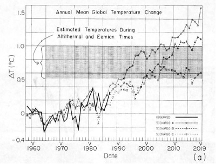
Figure 2: Projected global surface air temperature changes in Scenarios A, B, and C (Hansen 1988)
Notice that Michaels erased Hansen's Scenarios B and C despite the fact that as discussed above, Scenario A assumed continued exponential greenhouse gas growth, which did not occur. In other words, to support the claim that Hansen's projections were "an astounding failure," Michaels only showed the projection which was based on the emissions scenario which was furthest from reality.
Gavin Schmidt provides a comparison between all three scenarios and actual global surface temperature changes in Figure 3.
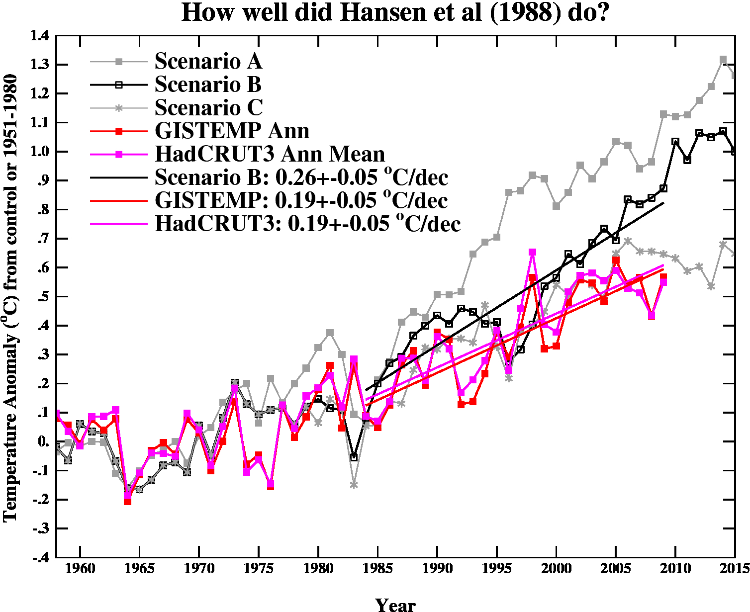
Figure 3: Hansen's projected vs. observed global temperature changes (Schmidt 2009)
As you can see, Hansen's projections showed slightly more warming than reality, but clearly they were neither off by a factor of 4, nor were they "an astounding failure" by any reasonably honest assessment. Yet a common reaction to Hansen's 1988 projections is "he overestimated the rate of warming, therefore Hansen was wrong."
In fact, when skeptical climate scientist John Christy blogged about Hansen's 1988 study, his entire conclusion was "The result suggests the old NASA GCM was considerably more sensitive to GHGs than is the real atmosphere." Christy didn't even bother to examine why the global climate model was too sensitive or what that tells us. If the model was too sensitive, then what was its climate sensitivity?
This is obviously an oversimplified conclusion, and it's important to examine why Hansen's projections didn't match up with the actual surface temperature change. That's what we'll do here.
Hansen's Assumptions
Greenhouse Gas Changes and Radiative Forcing
So which scenario was the most accurate representation? Figures 4 below provides the answer. The radiative forcings for Hansen's three scenarios were estimated using the simplified radiative forcing expressions from the 2001 IPCC report, based on the projected greenhouse gas atmospheric concentrations for Hansen's scenarios. The actual radiative forcing estimates are taken from Skeie et al. (2011).
Hansen et al. only modeled the temperature response to greenhouse gas changes (and a few simulated volcanic eruptions). So in his simulations, the greenhouse gas (GHG)-only forcing and 'all forcings' are the same. In reality, they are not, with the main non-GHG forcing involving human aerosol emissions, whose effects remain one of the biggest uncertainties in climate science.
In our analysis here, we're interested in the changes since 1988, particularly through 1998. The radiative forcing changes since 1988 are shown in Figure 4.
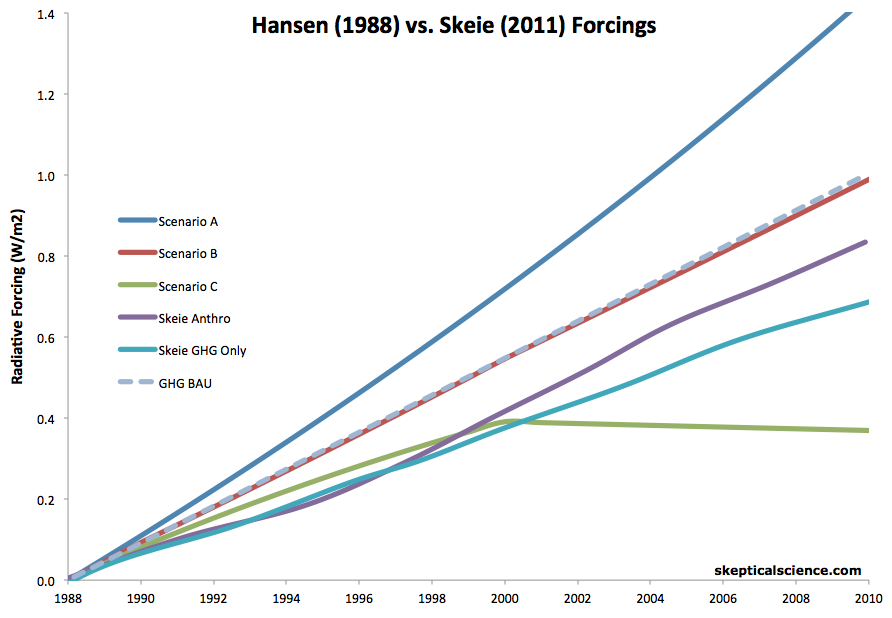
Figure 4: Radiative forcing changes (1988 to 2010) for the three emissions scenarios in Hansen et al. 1988 (dark blue [A], red [B], and green [C]) vs. Skeie et al. (2011) GHG-only (light blue) and all anthropogenic forcings (purple).
Both the GHG-only and net anthropogenic forcing changes between 1988 and 1998 were very close to Hansen's Scenario C, consistent with Figure 1 above, primarily due to the CFC emissions reductions as a result of the Montreal Protocol.
Recreating Michaels' Congressional Testimony Graphic
As Figure 4 shows, Hasen's Scenario B is currently closest to the actual forcing (according to Skeie et al.), but running about 16% too high (since 1988). Figure 5 reproduces Hansen's Scenario B with a 16% reduction in the warming trend, to crudely correct for the discrepancy between it and the actual radiative forcing. This might be what Michaels' graphic would look like if he were to give an accurate version of his presentation today:
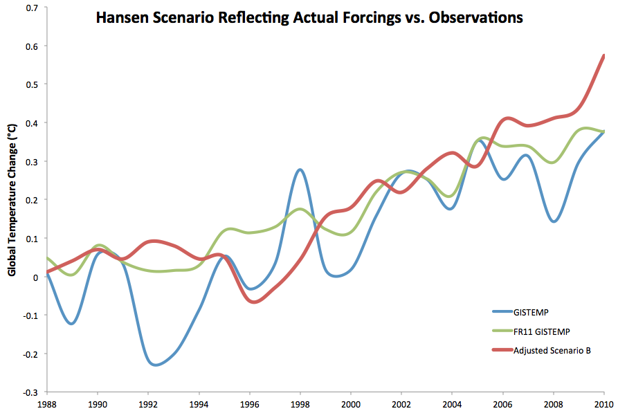
Figure 3: Observed temperature change (GISTEMP, blue) and with solar, volcanic and El Niño Southern Oscillation effects removed by Foster and Rahmstorf (green) vs. Hansen Scenario B trend adjusted downward 16% to reflect the observed changes in radiative forcings since 1988, using a 1986 to 1990 baseline.
In Figure 3 we've included both GISTEMP data, and GISTEMP with solar, volcanic, and El Niño Southern Oscillations removed by Foster and Rahmstorf (2011). The 1988 to 2010 trends are similar, 0.20°C per decade with the natural effects, 0.18°C per decade without. Scenario B has a 0.23°C per decade trend, but when removing a simulated volcanic eruption in 1996, the trend decreases to about 0.22°C per decade.
As the figure above shows, Hansen's 1988 model overpredicted the ensuing global warming. However, it only overpredicted the warming by approximately 15 to 25%, which is a far cry from the 300% overprediction claimed by Michaels in his 1998 congressional testimony.
Climate Sensitivity
Climate sensitivity describes how sensitive the global climate is to a change in the amount of energy reaching the Earth's surface and lower atmosphere (a.k.a. a radiative forcing). Hansen's climate model had a global mean surface air equilibrium sensitivity of 4.2°C warming for a doubling of atmospheric CO2 [2xCO2]. The relationship between a change in global surface temperature (dT), climate sensitivity (λ), and radiative forcing (dF), is
dT = λ*dF
Knowing that the actual radiative forcing was slightly lower than Hansen's Scenario B, and knowing the subsequent global surface temperature change, we can estimate what the actual climate sensitivity value would have to be for Hansen's climate model to accurately project the average temperature change.
What we find is that Hansen's results add to the long list of evidence that climate sensitivity is not low. As noted above, Hansen's model overpredicted the ensuing global warming thus far by approximately 15 to 25%. Thus if we estimate that the sensitivity of his model was 15 to 25% too high (which is an oversimplification, but will give us a reasonably accurate back-of-the-envelope estimate), this suggests the actual climate sensitivity is approximately 3.4 to 3.6°C for doubled CO2, which is close to the IPCC best estimate of 3°C.
The argument "Hansen's projections were too high" is thus not an argument against anthropogenic global warming or the accuracy of climate models, but rather an argument against climate sensitivity being as high as 4.2°C for 2xCO2, but it's also an argument for climate sensitivity being around 3°C for 2xCO2, which is consistent with the range of climate sensitivity values in the IPCC report.
Spatial Distribution of Warming
Hansen's study also produced a map of the projected spatial distribution of the surface air temperature change in Scenario B for the 1980s, 1990s, and 2010s. Although the decade of the 2010s has just begun, we can compare recent global temperature maps to Hansen's maps to evaluate their accuracy.
Although the actual amount of warming (Figure 5) has been less than projected in Scenario B (Figure 4), this is due to the fact that as discussed above, we're not yet in the decade of the 2010s (which will almost certainly be warmer than the 2000s), and Hansen's climate model projected a higher rate of warming due to a high climate sensitivity. However, as you can see, Hansen's model correctly projected amplified warming in the Arctic, as well as hot spots in northern and southern Africa, west Antarctica, more pronounced warming over the land masses of the northern hemisphere, etc. The spatial distribution of the warming is very close to his projections.
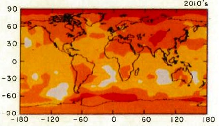
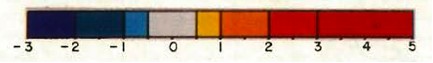
Figure 4: Scenario B decadal mean surface air temperature change map (Hansen 1988)
Figure 5: Global surface temperature anomaly in 2005-2009 as compared to 1951-1980 (NASA GISS)
Hansen's Accuracy
Had Hansen used a climate model with a climate sensitivity of approximate 3°C for 2xCO2 (at least in the short-term, it's likely larger in the long-term due to slow-acting feedbacks), he would have projected the ensuing rate of global surface temperature change accurately. Not only that, but he projected the spatial distribution of the warming with a high level of accuracy. The take-home message should not be "Hansen was wrong therefore climate models and the anthropogenic global warming theory are wrong;" the correct conclusion is that Hansen's study is another piece of evidence that climate sensitivity is in the IPCC stated range of 2-4.5°C for 2xCO2.
Last updated on 25 November 2016 by dana1981. View Archives


A minor note, inspired by re-reading Myhre et al 1998 on the radiative forcing of various greenhouse gases:
The forcing from a change in CO2 is estimated as F = α * ln(C/C0) - this is a shorthand fit to what is calculated from a number of line-by-line radiative calculations.
The 1990 constant, which is what I presume Hansen used in the 1988 model, had a constant α = 6.3, while Myhre et al 1998, using better radiative estimates, has α = 5.35. And that value has been used ever since in modeling estimations.
I suspect that difference in estimating radiative forcing may be responsible for much of the 4.2°C/doubling sensitivity Hansen 1988 (over)estimated, as opposed to the roughly 3°C/doubling value used now.
Tamino has updated Hansen's 1988 prediction by swapping in actual values of forcings (except volcanic) more recently than was done by RealClimate seven years ago. The forcings are closest to Hansen's Scenario C forcings. So actual temperatures should have been closest to Hanson's Scenario C model projection. Guess what?
Several obvious problems here.
First, Hansen's 1988 presentation was about emissions, as the Congressional record clearly shows. Actual global emissions look like Scenario A (if mainly because of China). Yes, the forcings in the model depend on concentrations, but the fact that methane or CO2 concentrations didn't do what the model expected are failures of Hansen 1988 to accurately model the relationship of emissions to concentrations. This is part of what critics have accurately labelled the "three-card monte" of climate science: make a claim, then defend some other claim while never acknowledging the original claim was false. This is not how good science is done.
Second, the graph purports to measure whether Hansen 1988 made accurate predictions, but it doesn't start in 1988. To show the hindcast (which the model was deliberately tuned to!) is another kind of three-card monte.
One can quibble with the choice of the GISS surface temperature record, given that Hansen himself administered it, but the divergence from satellite doesn't really affect the conclusions, so suffice it to note the 1988 prediction looks slightly worse using UAH or RSS.
Another minor quibble is that the article is now somewhat out of date — we're well into the 2010s and the predicted warming is still not materializing. This also makes the prediction slightly more wrong.
Last, and most risibly, the resemblance of actual temperatures to Scenario C predictions is now being held up as vindication. Even if that were defensible on the merits, it would certainly have come as a great shock to Hansen and his audience in 1988. Imagine a time traveler arriving from 2014, barging into Senate hearings brandishing the satellite record and yelling "Hansen was right! Look, future temperatures are just like Scenario C!" The obvious conclusion would have been "oh good, there's no problem then."
As this is an advocacy site, I do not expect these errors to be corrected, I merely state them for the record so visitors to the site can draw their own conclusions.
TallDave, you say: "Actual global emissions look like Scenario A (if mainly because of China)."
Except, that if you read the link in the post directly above your own, you find information to the contrary. Perhaps you'd care to present your alternative data, that demonstrates that emissions(or even better, forcings) do in fact look like scenario A.
TallDave - Um, no. Emissions more closely tracked Hansens Scenario C in terms of total forcings, as shown here.
[Source]
Those emission scenarios were "what-if" cases (not predictions) of economic activity, which are not in and of themselves climate science. Any mismatch of between those scenarios and actual events would only be an issue if Hansen was writing on economics, not on climate. He could hardly have predicted the Montreal Protocols on CFC's, for example.
"suffice it to note" - Strawman WRT to satellite temps, as Hansen was discussing surface temperatures and not mid-tropospheric temperature; you're attempting to attack something that wasn't discussed in his paper.
Yes, that 1988 paper is now out of date. Amazingly, though, it's frequently brought up and attacked on 'skeptic' websites, as if it represented current information - so it's quite reasonable to discuss these attacks on SkS as the current denial myths they are.
The real question is whether the model performs well in replicating temperatures given particular forcings - and since it does, it was a pretty decent model. The predictions of the paper were not "either Scenario A, B, or C will occur", but rather "Given a set of stated emissions, here's what the temperatures are likely to be", establishing a relationship between concentrations of forcing agents, and temperatures.
The major problem with his 1988 predictions came down to slightly too high a sensitivity to forcings (4.2 C/doubling of CO2, rather than ~3.2). This was strongly influenced by the radiative models and available data of the time, with the simplified expression at the time for CO2 forcing being 6.3*ln(C/C0). That constant was updated a decade later by Myhre et al 1998 to 5.35*ln(C/C0). Hansen used the data he had at the time, and his sensitivity estimate was a bit high.
If Hansen had time-traveled a decade and used that later estimate, his input sensitivity would have been ~3.57 C/doubling of CO2 - and his emissions to temperature predictions for the next 25 years would have been astoundingly accurate.
Your comment is a collection of strawmen arguments, and rather completely misses the point of the Hansen 1988 paper. It drew conclusions regarding the relationship of greenhouse gases and temperatures, not on making economic predictions. If you're going to disagree with it, you should at least discuss what the paper was actually about.
Talldave @20 claims, "Hansen's 1988 presentation was about emissions, as the Congressional record clearly shows."
Conveniently he neglects to link to the congressional record, where Hansen says:
Curiously, he makes no mention of emissions at all, when enumerating his three conclusions.
Later, and talking explicitly about the graph from Hansen et al (1988) which showed the three scenarios, he says:
Hansen then goes on to discuss other key signatures of the greenhouse effect.
As you recall, Talldave indicated that Hansen's testimony was about the emissions. It turns out, however, that the emissions are not mentioned in any of Hansen's three key points. Worse for Talldave's account, even when discussing the graph itself, Hansen spent more time discussing the actual temperature record, and the computer trend over the period in which it could then (in 1988) be compared with the temperature record. What is more, he indicated that was the main point.
The different emission scenarios were mentioned, but only in passing in order to explain the differences between the three curves. No attention was drawn to the difference between the curves, and no conclusions drawn from them. Indeed, for all we know the only reason the curves past 1988 are shown was the difficulty of redrawing the graphs accurately in an era when the pinacle of personal computers was the Commodore Amiga 500. They are certainly not the point of the graph as used in the congressional testimony, and the congressional testimony itself was not "about emissions" as actually reading the testimony (as opposed to merely referring to it while being carefull not to link ot it) actually demonstrates.
Ironically, Talldave goes on to say:
Ironical, of course, because it is he who has clearly, and outragously misrepresented Hansen's testimony in order to criticize it. Where he to criticize the contents of the testimony itself, mention of the projections would be all but irrelevant.
As a final note, Hansen did have something to say about the accuracy of computer climate models in his testimony. He said, "Finally, I would like to stress that there is a need for improving these global climate models, ...". He certainly did not claim great accuracy for his model, and believed it could be substantially improved. Which leaves one wondering why purported skeptics spend do much time criticizing obsolete (by many generations) models.
Tristan/KR — as I pointed out in my original post, you're making the usual mistake of confusing "emissions" for "concentrations" or "forcings." Again, Hansen made predictions explicitly based on emissons to Congress, see his full remarks in the pdf below. Indeed, the purpose of the hearing was to persuade Congress to take action on emissions.
Emissions (especially of CO2) rose like Scenario A. Don't take my word for it, ask the EPA:
http://www.epa.gov/climatechange/images/ghgemissions/TrendsGlobalEmissions.png
Tom: Here is the entire text of Hansen's remarks. Note this passage:
"We have considered cases ranging from business as usual, which is Scenario A, to draconian emissions cuts, Scenario C..."
http://image.guardian.co.uk/sys-files/Environment/documents/2008/06/23/ClimateChangeHearing1988.pdf
Surely no one seriously argues there were draconian cuts in emissions after 1988.
"Which leaves one wondering why purported skeptics spend do much time criticizing obsolete (by many generations) models."
Obviously because they're the only ones that can be tested on any meaningful time scale. Contra this site, the ability of a model to hindcast a highly complex phenemonen gives little confidence in its forecast (something painfully well-known in other fields).
Tom C is not saying Hansen did not mention emissions, just that they were not central to Hansen's testimony, and did not figure into his main points which were about whether observed warming had happened and whether it could be linked to GHGs and therefore be tied to humans.
What matters in any climate model is the GHG forcing, which is a function of concentrations. Emissions affect that, but indirectly and in a lagged fashion, so the timing of emissions and their makeup affect the realized concentration.
Hansen could not know that methane would show it's odd pattern over time, that CFC's production would be curtailed by the Montreal protocol a few years later, and that the Soviet bloc would collapse, along with it's industry. Current emissions of CO2 in particular could be pretty high, but if the timing of those emissions was backloaded, you will not see the overall forcing.
You're argument for your fixation on old models doesn't ring true. More sophisticated GCMS produced later have plenty of new data they can be compared against. Nobody gauges what you can do with a current computer based on what the Commodore Amigo could do in 1988. That is a crazy idea.