Climate Science Glossary

Term Lookup

Enter a term in the search box to find its definition.

Settings

Use the controls in the far right panel to increase or decrease the number of terms automatically displayed (or to completely turn that feature off).

Term Lookup

Settings


All IPCC definitions taken from Climate Change 2007: The Physical Science Basis. Working Group I Contribution to the Fourth Assessment Report of the Intergovernmental Panel on Climate Change, Annex I, Glossary, pp. 941-954. Cambridge University Press.

Home Arguments Software Resources Comments The Consensus Project Translations About Support

Twitter Facebook YouTube Mastodon MeWe

RSS Posts RSS Comments Email Subscribe


Climate's changed before
It's the sun
It's not bad
There is no consensus
It's cooling
Models are unreliable
Temp record is unreliable
Animals and plants can adapt
It hasn't warmed since 1998
Antarctica is gaining ice
View All Arguments...


Username
Password
New? Register here
Forgot your password?

Latest Posts

Archives

Radiative Balance, Feedback, and Runaway Warming

Posted on 26 February 2012 by Chris Colose

Skeptical Science has previously discussed the topic of feedbacks and why the existence of positive feedbacks (i.e., those feedbacks that amplify a forcing) do not necessarily lead to runaway warming, or even to an inherently "unstable" climate system.  I also wrote on it at RealClimate (and Pt. 2). This was brought up again in Lord Christopher Monckton's response to SkepticalScience, where he asserted:

"First, precisely because the climate has proven temperature-stable, we may legitimately infer that major amplifications or attenuations caused by feedbacks have simply not been occurring...A climate subject to the very strongly net-positive feedbacks imagined by the IPCC simply would not have remained as stable as it has."

I wanted to revisit the subject in order to take a different approach on the subject of positive feedbacks.  This involves the relationship between Earth's surface temperature and outgoing infrared radiation (the energy Earth emits to space). Determining how the outgoing longwave radiation (OLR) depends on surface temperature and greenhouse content is a fundamental determinant to any planetary climate.

I'll begin with very trivial, ideal cases, and then slightly build up in complexity in order to relate the problem to climate sensitivity.  By the end, it should be clear why positive feedbacks can exist that inflate climate sensitivity but do not necessarily call for a runaway warming case.  We'll also see a scenario, commonly discussed by planetary scientists, in which it does lead to a runaway.

First, we begin with the simplest case in which the Earth has no atmosphere and essentially acts as a perfect radiator. In this case, the outgoing radiation is given by the Stefan-Boltzmann equation OLR=σT4. T is temperature. σ is a constant, so the equation means that the outgoing radiation grows rapidly with temperature, (to the power of four) as shown below.

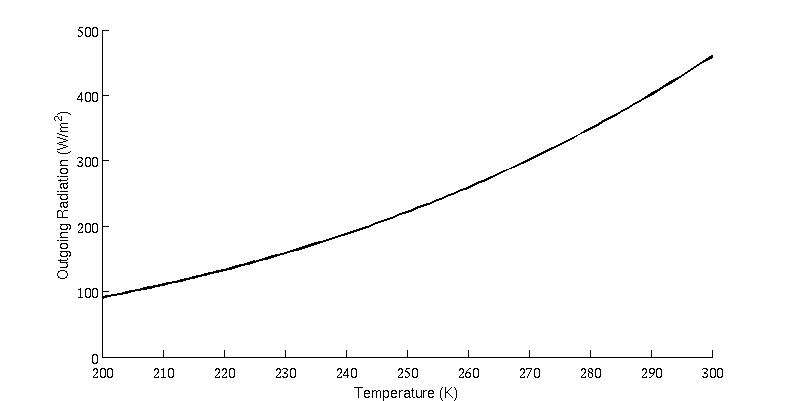
Figure 1: Plot of OLR vs. Surface temperature for a perfect blackbody


In the next case, suppose that we add some CO2 to the atmosphere (400 ppm).  The atmosphere here is completely dry (and therefore no water vapor feedback).  In this example, the addition of CO2 will reduce the OLR for any given temperature, since the atmosphere absorbs some of the exiting energy.  This is displayed with the red curve in Figure 2 (the black curve is from above for reference).

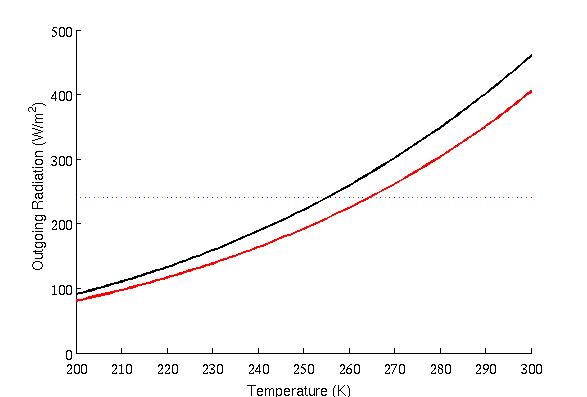
Figure 2: Relationship between OLR and surface temperature for a blackbody (black curve) and with 400 ppm CO2 (red curve).  The horizontal line is the absorbed solar radiation.

Also plotted in Figure 2 is a horizontal line at 240 W/m2, which corresponds to the amount of solar energy that Earth absorbs.  In equilibrium, the Earth receives as much solar energy as it does emit infrared radiation.  Therefore, in the above plot, the points at which the horizontal line intersect the black/red lines will correspond to the equilibrium climates in this model.  Note that the red line makes this intersection at a higher surface temperature, which is the greenhouse effect.

Now let's step up the complexity a bit.  We'll throw in some water vapor into the model, but not just a fixed amount of water vapor.  This time, we'll also let the water vapor concentration increase as temperature increases.  Water vapor is a good greenhouse gas, so now the infrared absorption grows with temperature. This is the water vapor feedback.  The blue line in the next  figure is the OLR for a planet with the same 400 ppm CO2, in addition to this operating feedback.

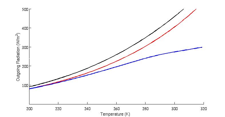
Figure 3: Relationship between OLR and surface temperature, as above, but with a constant relative humidity atmosphere (blue line, implying increasing water vapor with temperature)

In this figure, we see that the OLR does not depend very much on the water vapor at low temperatures.  This makes sense, because at temperatures this cold (such as during a snowball Earth), there is so little water vapor in the air.  However, at temperatures similar to the modern global mean and warmer, the OLR drops tremendously and the the T4 dependence instead becomes much flatter.  We'll get a more clear picture of that means for climate sensitivity in the next diagram.

In the next diagram, I've removed the red curve for convenience.  But I've added two horizontal lines this time.  You can think of this as two possible values for the incoming solar radiation. 

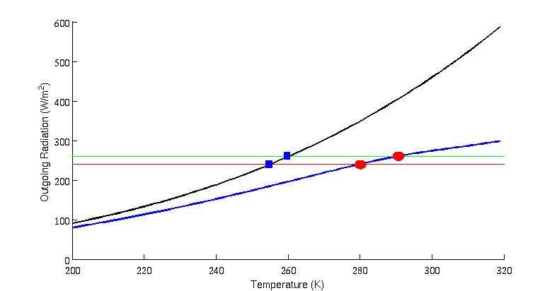
Figure 4: OLR vs. surface temperature for a blackbody (black curve) and an atmosphere with CO2 and a water vapor feedback (blue curve).  The horizontal lines give two values for the absorbed incoming solar radiation, and the colored shapes give possible equilibrium points.  On the trajectory where water vapor exists, sensitivity is enhanced because the temperature difference between the two red circles (as sunlight goes up) is greater than the difference between the two blue squares.

To interpret Figure 4, suppose that we increase the amount of sunlight that the Earth gets, which means we jump from the red to the green line in the above figure.  If the Earth were a blackbody (black curve) then the temperature change that results from this would just be the difference between the values at the two blue squares.  However, in a world with a water vapor feedback, the temperature difference is given by the distance between the two red circles.  We can infer from this that water vapor has increased climate sensitivity, yet it did not cause a runaway warming effect.

Now let's consider one more case.  Notice in the previous diagram that at very high temperatures, the OLR starts to flatten out, and indeed eventually can become almost flat.  This is due to the rapid increase in water vapor (and infrared absorption) as temperature goes up.  But suppose we pump up the amount of sunlight that the Earth gets to much higher values than in the last figure.  This new value is shown by the horizontal green line in the figure below.

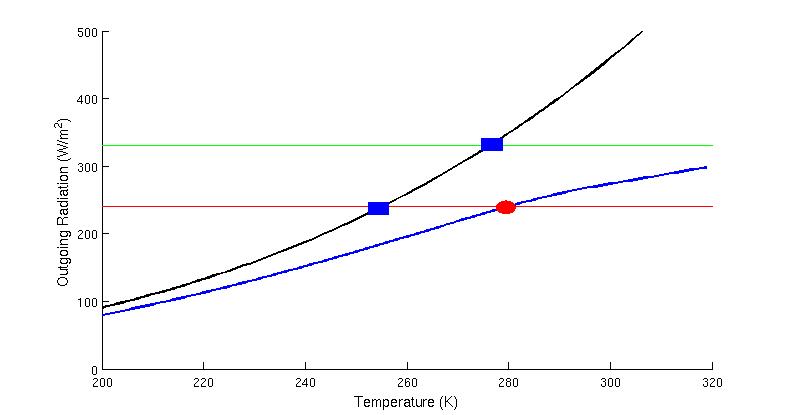
Figure 5: As above, but the green line corresponds to higher incoming solar radiation.

Once again, if we follow the black curve (with no atmosphere), then we get an expected increase in temperature as the amount of sunlight goes up.  But if we follow the blue curve (the system with an operating water vapor feedback), then something strange happens. 

At some point the OLR becomes so flat, that it can never increase enough to match the incoming sunlight.  In this case, it actually becomes impossible to establish a radiative equilibrium scenario, and the result is a runaway greenhouse.  This is the same phenomenon planetary scientists talk about in connection with the possible evolution of Venus or exoplanets outside our solar system.  The system will only be able to come back to radiative equilibrium once the rapid increase of water vapor mass with temperature ceases, which in extreme cases may not be until the whole ocean is evaporated.

From these figures, we can readily see the fallacy in "positive feedbacks imply instability" type arguments.  There is in fact a negative feedback that always tends to win out in the modern climate.  This is the increase in planetary radiation emitted to space as temperature goes up.  Positive longwave radiation feedbacks only weaken the efficiency at which that restoring effect operates.  Instead of the OLR depending on T4, it might depend on T3.9, or maybe even T3 at higher temperatures; eventually the OLR becomes independent of the surface temperature altogether.  I haven't discussed shortwave feedbacks, such as the decrease in albedo as sea ice retreats.  That only raises the position of the horizontal lines slightly, allowing for a warmer equilibrium point, but in no way compromises the argument.

In fact, the same sort of argument can be applied if we let the albedo vary with temperature (and so the absorbed solar radiation is no longer given by a horizontal line).  The opposite extreme, a snowball Earth, can then be thought of as a competition between the decreased longwave radiation to space as the planet cools, and the increased reflection as the planet brightens (when the ice line is advancing toward the equator).  As with a runaway greenhouse, it's not inevitable that this occurs, as is evident from times in Earth's history when ice advanced but did not reach the equator. 

As a final note, it's worth mentioning that it is virtually impossible to trigger a true runaway greenhouse in the modern day by any practical means, at least in the sense that planetary scientists use the word to describe the loss of any liquid water on a planet.  The most realistic fate for Earth entering a runaway is to wait a couple billion years for the sun to increase its brightness enough, such that Earth receives more sunlight than the aforementioned outgoing radiation limit that occurs in moist atmospheres.  None of this means that climate sensitivity cannot be relatively high however. 

Note: Except for the first graph, all computations here were done using the NCAR CCM radiation module embedded within the Python Interface for Ray Pierrehumbert's supplementary online material to the textbook "Principles of Planetary Climate."  The lapse rate feedback is included as an adjustment to the moist adiabat. I've assumed near-saturated conditions are maintained (constant 100% relative humidity) with temperature, although the argument is qualitatively similar with lesser RH values.

This post has been adapted into the Advanced rebuttal to "Positive feedback means runaway warming"

0 0

Printable Version  |  Link to this page

Comments

1  2  Next

Comments 1 to 50 out of 99:

  1. This is a fantastic explanation. I had spent a little bit of time thinking about this problem, but now reading this post I realize I didn't yet have the information needed to reason this through. Thanks!
    0 0
  2. So obvious, once clearly explained. Thank you, Chris.
    0 0
  3. Good article.
    0 0
  4. Fantastic article. Now I can realy see the GH effect in much better perspective. Few questions jump: Are those curves a true representatives of our real earth or just exemplary? If the former, can we say by how much the green and red horiz lines are appart when comparing recent solar energy with meander minimum during LIA? Then, what are the angles of intersection of red curve (CO2 only) and blue curve (CO2+H2O) with the current solar radiation line? Finally, if red curve represents 400ppmCO2 we have right now how far above the 280ppm curve would be? I'm asking those questions, because I want to have the feeling about the relative magnitude of the three forcings (solar, CO2 & H2O) we are talking about in this model. Thanks.
    0 0
  5. That explanation sure deserves a thank-you. Really nice read. Interesting chuckle over how we get trapped by our frameworks. When the blackbody was given a thin CO2 atmosphere, 'say 400ppm' ... if it's the only element in the atmosphere it's 1,000,000ppm, isn't it? The density equivalence starts with 1.977 g/l (gas at 1 atm and 0 °C) ... but I had to look it up. Interesting that at 25dC, the density drops to 1.799g/L.
    0 0
  6. Very nice thank you. I've read some stuff that mentions the adiabatic lapse rate. I suspect that this is part of the explanation above but left out for the sake of simplicity. Could you do another post where you expand on this part of the picture?
    0 0
  7. Nicely done! I have the same questions as Chriskoz and look forward to seeing your answers.
    0 0
  8. 4, chriskoz, 7, Pirate, I'll leave it to Chris to give you his answer, but just off the cuff, as he stated in his closing note he used the freely available online material that Ray Pierrehumbert provides for use with his book "Principles of Planetary Climate." Along those lines, that model is complex enough to include things you've never even considered, but still simple enough to run on your desktop in an interpreted language like Python, and for the code to be easily understood by anyone who follows his course by reading the book, doing the problems and working directly with the model. So the point is... it's a teaching model, designed to demonstrate concepts. It's accurate enough to show how the pieces fit together, but not to use as a model for getting specific values (such as "the runaway point" for our planet).
    0 0
  9. John Brookes at 23:20 PM on 25 February, 2012 You can also check David Archer's lecture about the lapse rate. It's part of a more comprehensive course on Global Warming for non-science undergrads.
    0 0
  10. 9. Alexandre The David Archer video link to the individual lecture, or links to any lectures from the "comprehensive course" webpage which I can get to, that you gave in your comment don't work for me. Maybe you have access to them at those links after logging in somewhere. What does work for me here in Seattle is to go to the UChicagoNews Mindonline PHSC 13400: Global Warming page and select lectures from there. The lecture on the lapse rate you were drawing attention to is lecture 9.
    0 0
  11. If you follow the links I gave I just discovered you get video and no sound, at least this machine doesn't. The lectures are on Youtube where they don't work as well.
    0 0
  12. David Lewis Thanks for pointing it out. The link I gave above is for download of the video, which is pretty big (241MB or over 30 minutes in my not-so-great internet connection). Your link seems to be more practical, and works fine for me, with video and sound.
    0 0
  13. owl905- Actually there is background non-greenhouse gas imposing a surface pressure of modern-day 1000 millibars, with CO2 mixed into that. There is no methane, ozone, or other GHGs in these experiments. John Brookes- The adiabatic lapse rate is just the temperature structure that most of the atmosphere relaxes to (in the vertical) due to the properties of convection. chriskoz- Actually the model is quite good, but it is one-dimensional, a crude global average without cloud feedbacks, so it's not a GCM or suitable for getting a precise handle on sensitivity. Results from output of this sort have been used in the literature however, so I feel justified in using it here.
    0 0
  14. Nice explanation. Thanks Chris. It is the exponential characteristic of the WV feedback that I find hardest to communicate to people. Your graphs, especially Figure 5, demonstrate this quite clearly.
    0 0
  15. Thanks for the clear and informative explanations. Thinking about various variables that affect sensitivity, I'm reminded of Richard Alley's incredible 2009 AGU lecture "The Biggest Control Knob: CO2 in Earth's Climate History" . It appears the 11-year solar cycle will cause greater temperature swings (within an equilibrium system) when the temperature is higher, lets say due to increased atmospheric CO2. Will this make future weather events more chaotic or less "average" (whatever is the new climatic average)? In our current not-in-equilibrium Earth system, the effects of the recent extended solar minimum (plus increased aerosols & La Nina) appear to have virtually countered temperature increases due to increasing CO2. I've read someplace that climate scientists are functionally certain that new global surface temperature records will occur within several years, at the latest. I presume this is because of the influence of both increasing CO2 and increasing solar radiation, regardless of what happens with ENSO or air polution. (SkS article about Dr. Alley can be found here.)
    0 0
  16. Chris Colose, Well done! ... I am a chemical engineer. It is beaten into our heads to relate things with graphs as doing so shows relationships so well. As of yet, I've never seen anyone explain 'sensitivity' so well as you have done. Sensitivity is simply the 'gain' or 'multiplier' that relates a change in an independent variable (i.e. forcing, such as CO2) to a change in the dependent variable (temp). In formula form: dT = Sensitivity x dCO2. Essentially, S is the SLOPE on a graph. (For a graph formatted with Temp on the x- axis as in the article, Sensitivity would actually be '1/slope'.) And, WOW!, your article shows this visually so well! It clearly shows how a more horizontal sloped curve (for Flux vs Temp formatted graphs) versus a more vertically sloped curve result in HIGHER sensitivities. This is the kind of technical (but yet simple) explanation that will turn the heads of the more technically astute minds out there (assuming they are the least bit open-minded)! This is the kind of stuff that might get them to say, "Oh! Now I get it!" Like, @4 chriskoz and @7 Pirate mentioned, I would propose a PART-2 follow-up article which I think would knock this whole thing over the fence. Then, I would feel fully ready to explain the science of global warming amply loaded with the needed ammunition that could NOT be refuted. I can only wonder if such an addendum would also be universally helpful. Here is the suggestion: After Fig.3, I would take the article on a slightly different course. For the next graph, I would show two RED curves; one for 250ppm (pre-industrial) and another for 500ppm (give a hypothetical year, 2065). Why 250 & 500 curves? These CO2 values work well with the typical scientific talk of doubling CO2 and how such a doubling impacts temperature. Plus it shows realistic resulting temperatures for a starting point (pre-ind) CO2 and not-so-far-away (2065) CO2. ... Leave the horizontal line at 240 W/m2 (at this point in the article assume albedo differences and solar cycle variances are still neutral). With these two CO2-only RED curves, I would expect the difference in equilibrium temp to be ~1.0 - 1.2K, which I have read on this site as the expected dTemp for doubling of CO2 with NO other feedbacks mixed in. Then, on this same graph, add two BLUE curves representing the average Relative Humidity earth conditions, one at 250ppm CO2 and the other at 500ppm CO2. I assume the '500ppm w/RH' curve will simply be shifted down below the '250ppm w/RH' curve (you would know the exact particulars on this better than I). If you look at the present Fig.3, I see how, at 200K, the RED curve is shifted vertically down below the BLACK curve, and the BLUE curve (at this 200K) also "starts" at this same point (at this trace humidity state). For the 250ppm & 500ppm RED & BLUE curves, they will simply start (at the 200K temp) at two different vertical shifts down from the BLACK curve, with the 500ppm curve simply being 'LOWER' than the 250ppm curve (probably by the same porportional vertical distance). Then, when these curves move to the right from this starting point (200K), they will cross the 240W/m2 horizontal line at their various equilibrium temperatures. [Slight diversion: WOW, your article is so COOL how it visually explains these changes in the equilibrium point. With your clear graphs, any technically oriented person would instantly understand & get your point and realize its significance in a heartbeat!] Since the two BLUE curves are so much flatter (i.e. or lower angle, or read higher sensitivity), the horizontal distance between the two BLUE curves will be much greater than the horizontal distance for the RED curves, i.e. a much higher sensitivity. Therefore, the 1.0-1.2 dT for doubling of CO2 alone turns into ~3.0dT when adding in the humidity feedback. ... This would really help explain the positive feedback of humidity added on top of doubling CO2 alone. After this, I would take the article the direction as proposed by @4 chriskoz. This graph could show the impact on Temp caused by an extreme change in solar radiation, such as during the Maunder Minimum, but I would like to see the article stay more applicable to today's typical solar cycles. Therefore, I would setup this next graph to show the resulting dT between 1) a LOW POINT on our current measured SOLAR CYCLES and 2) a HIGH POINT on our current SOLAR CYCLES. I don't know what the difference in average, earth-surface, net input W/m2 for these two points amounts to ... ~0.25W/m2??? But whatever it is, show these two horizontal lines super-imposed on a "detailed" view of the graph ('detailed' so to better see the dT impact). I expect this equilibrium dTemp impact to be roughly 10% (or less) than that for the CO2 doubling w/ RH impact (~3.0dT). I recall reading on this site that modern variances in solar radiation amounts to (at most) 1/10th that of human induced CO2 changes. owl905: Your point about 400ppm (or 1,000,000 ppm) is NOT a small point! And, the article probably needs to be tweaked a bit in its wording to assure absolute accuracy. The greenhouse effect of CO2 can NOT be ONLY a function of its %concentration (PPM) amongst the rest of gases. Instead, it HAS to be a function of actual #moles per unit volume of CO2 in the atmosphere (or, more clearly for most people, MASS per unit volume). These two are not the same; a given PPM does NOT mean a set MASS/volume concentration. For example, imagine an atmosphere that only had 1/10 the mass (in the entire atmosphere) of N2 and O2 (these being non-greenhouse gases). Then, let's only add CO2 to this hypothetical atmosphere; thus it is the ONLY greenhouse gas in the atmosphere. But, let's add the CO2 to a %concentration of 400ppm, then obviously the mass of CO2 (per unit volume) would be 1/10 of our present atmosphere. There is NO WAY this 1/10 mass/volume CO2 atmosphere could have the same greenhouse effect as our present atmosphere. The point here is that the key driving variable HAS to be MASS/volume NOT % of molecules which, technically, is all that PPM really states. Therefore, the key variable defining greenhouse effect is not PPM, but actually mass/volume or molecules/volume (however you want to express it). But, this detail is getting TOO technical for most people to understand & it deviates from the usually 'talk' of defining the greenhouse effect as a function of PPM. So, I would simply say (for Fig.2) that you would first "flood the atmosphere with present day quantities of N2 and O2, then add CO2 to the concentration of 400PPM". Then, explain that the N2 & O2 cause NO greenhouse effect, so you have created an artifical atmosphere that has a CO2-only greenhouse effect that would mimic today's atmospheric "concentration" of 400ppm of CO2 (this being your original intention in Fig.2) ... without explaining the detail that this also means that this hypothetical atmosphere would also have the same mass/volume concentration of CO2 as today's atmosphere. This slight wording tweak ("400ppm in the same N2 & O2 atmosphere as per today's atmosphere") would then be technically fully accurate and defendable. Sorry for LONG comment. I tend to get too windy.
    0 0
  17. I'll add my voice to the chorus on clarity! On a side note, isn't it interesting to see how Monckton thinks the positive feedbacks play into this? According to his wording, the IPCC imagines them. Pretty sure that these actually originate from physicists and other earth scientists who study the atmosphere, write the literature on it, and that literature is then eventually summarized by the IPCC. Even the models they use in the report are set up and run by scientists for their own purposes, not for making IPCC reports. It betrays some of the mindset that it takes to shrug off such a strong, facts-based, scientific consensus: "This must not be coming from the majority of working scientists trying to make sense of the planet, it must be coming from the United Nations' political machinery and their need to support the Big Government Wealth Redistribution Agenda!" or something along those lines.
    0 0
  18. sauerj- I wouldn't have thought that the article was that exciting, but glad I could help! I didn't show graphs with different CO2 concentrations because you'd barely see the difference between what I did, and say, an 800 ppm experiment. Keep in mind that the forcing for 2xCO2 is something like 4 W/m2 and I'm plotting the y-axis on these graphs over a range of many hundreds of W/m2, so it won't show up well unless you go to CO2 levels much higher than we're really worried about for future global warming. And it turns out that the OLR threshold at which it start to level off and become independent of temperature doesn't depend too strongly on the CO2 concentration.
    0 0
  19. Very clear explanation, and excellent graphs, thanks. One quibble: From these figures, we can readily see the fallacy is "positive feedbacks imply instability" type arguments. ... should read "the fallacy in"
    0 0
  20. corrected- thanks
    0 0
  21. This is an areas where semantics and precise meanings DO matter. Many climate scientists use the term "net positive feedback" to mean that all second order feedbacks other than the Stefan-Boltzmann radiation term are positive. That is quite different than a true net positive feedback, where the positive feedbacks are larger than the negative feedback of ithe increase in radiation caused by the increase in temperature.
    0 0
  22. @Saurj 16 - thanks for the expansion. For the purpose of ChrisC's review, maybe ppmv would work. @ChrisC - After three rounds of Moncton and the greatest extinction in the history of earth, explaining blackbody, sensitivity, and the temperature/gas dance with a few simple graphs ... is a grand slam. Maybe you could send this to the guys at The Big Bang Theory ... even Penny might get this one.
    0 0
  23. Charlie A @21, I believe climate scientists use the term "net positive feedback" to mean that the feedback including the Stefan-Boltzmann radiation term is positive, ie, that the temperature response of the initial forcing plus the feedback is larger than the temperature response of the initial forcing alone.
    0 0
  24. Tom Actually Charlie is correct here. Climate scientists usually don't define the Stefan-Boltzmann response as a feedback whatsoever, but rather as the baseline relative to how other feedbacks are referenced. Take the following image for example (from Roe, 2009): Roe 2009 Here the y-axis is the feedback factor,f, typically associated with the equation 1/1-f. Climate sensitivity is proportional to 1/1-f. More specifically it is *equal to* CS=b/1-f where b is the response you'd get in a system that only had the Stefan-Boltzmann response operating. Thus, in the limit where we have no feedbacks, f=0 and the equation reduces to CS=b. That is, you'd get the response from just the Stefan-Boltzmann response. In the above graph, the "all" feedback factor is positive, f=0.6 or so. This means that CS = b/0.4 = 2.5b (i.e., climate sensitivity is inflated by a factor of 2.5). Note however that the Stefan-Boltzmann response is not included in the graph.
    0 0
  25. Thanks for an informative and well written article. It is helping me clarify my understanding and thinking about this issue, and will likely be more helpful when I reread it. Is there an editing oversight in the caption for Figure 4, where the caption says "blue circles," while the figure shows and text states "blue squares?"
    0 0
  26. fixed, thanks
    0 0
  27. Regarding your statement: "it's worth mentioning that it is virtually impossible to trigger a true runaway greenhouse in the modern day by any practical means, at least in the sense that planetary scientists use the word to describe the loss of any liquid water on a planet" Hansen's discussed this issue in his December 2008 AGU Bjerknes Lecture. He also addressed this topic in Chapter 10 "The Venus Syndrome" in his book "Storms of My Grandchildren". He says he decided to bring the Venus Syndrome into the discussion because "it seems possible that strategic changes to fossil fuel use will not be adopted", i.e. civilization will burn every bit of fossil carbon that can be extracted from the Earth's crust. "So we had better examine what may happen if we push the planet beyond its tipping point". He says in the explanation in his book that Venus once had abundant water vapour in its atmosphere and "probably" had oceans. As the Sun brightened from its 30% less bright early solar system state, Venus heated up, "and the strong greenhouse effect of water vapor amplified the warming. Eventually a 'runaway' greenhouse effect occurred, with the ocean boiling or evaporating into the atmosphere". As the water vapor dissociated when it encountered UV at the top of the atmosphere, H escaped into space leaving O to combine with the C that had "baked out" of the crust until the atmosphere was 97% CO2 at a pressure of 90 bars. He says this theory is confirmed by the enrichment of heavy hydrogen, i.e. deuterium, on Venus today which is ten times more abundant there relative to normal hydrogen than on Earth or in the Sun. Ergo Venus was once wet. "So Venus had a runaway greenhouse effect". He displayed this graph in the Bjerknes Lecture as well as in his book: 
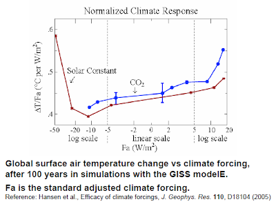
The graph, he says, "illustrates results of experiments with two different climate forcings: changing atmospheric carbon dioxide and changing brightness of the sun". "Qualitatively, this is the behavior that we know must occur: A sufficient negative forcing causes a runaway snowball Earth condition, with freezing temperatures over the entire planet, while a sufficient positive forcing causes a runaway greenhouse effect. We know that this U-shaped curve is correct - the question is, at what forcings do the sharp upturns to runaway conditions occur?" He suggests "that the forcings needed to reach snowball Earth or runaway greenhouse conditions are no more than 10 to 20 W/m2 when solar irradiance or CO2 change are defined as the forcing". After some discussion of the evolution of climate science, he says: "Now we are ready for the important part - trying to figure out how close we are to the climate forcing that will cause a runaway greenhouse effect. Until recently I did not worry too much about that", because much more CO2 had been in ancient atmospheres, "probably a few thousand parts per million", more than burning all the fossil fuels could produce. "So we should be safe, right? Wrong, unfortunately". 250 million years ago the sun was 2% dimmer, which is an equivalent forcing change to a doubling of CO2. "So if the estimated amount of CO2 250 million years ago was 2,000 ppm, it would take only about 1,000 ppm of CO2 today to create a climate equally as warm". But this is not the biggest factor, he says. Some estimates of early Cenozoic CO2 are as low as 1,000 ppm. He points to a Zeebe, Zachos, and Dickens 2009 paper which he quotes from: "Our results imply a fundamental gap in our understanding of the amplitude of global warming associated with large and abrupt climate perturbations". His estimate of Cenozoic CO2 depended on there not being this fundamental gap. If Cenozoic climate sensitivity was greater than 3 degrees C for 2x CO2 it favors lower estimates for how much CO2 there was. "The PETM results would be easier to understand if the baseline CO2, prior to the PETM warming was closer to 500 ppm. But even so, the magnitude of the PETM warming implies a climate sensitivity greater than 3 degrees for doubled CO2". He notes: "if we burn all the fossil fuels, the forcing wil be at least comparable to that of the PETM, but it will have been introduced at least ten times faster. The time required for the ocean to respond to this forcing is only centuries. Thus, carbon cycle diminishing feedbacks will not significantly reduce the ocean warming. The warming ocean can be expected to affect methane hydrate stability at a rate that could exceed that in the PETM, where the rate of change was driven by the speed of the methane hydrate climate feedback, not by the nearly instantaneous introduction of all fossil fuel carbon". "Carbon cycle diminishing feedbacks, which were important for keeping Earth away from runaway conditions during paleoclimate global warming events, are not likely to be as effective in drawing down atmospheric CO2 during the very rapid burning of fossil fuels by humanity". "It is difficult to imagine how the methane hydrates could survive, once the ocean has had time to warm. In that event a PETM-like warming could be added on top of the fossil fuel warming. After the ice is gone, would Earth proceed to the Venus syndrome, a runaway greenhouse effect that would destroy all life on the planet, perhaps permanently? While that is difficult to say based on present information, I've come to conclude that if we burn all reserves of oil, gas and coal, there is a substantial chance we will initiate the runaway greenhouse. If we also burn the tar sands and tar shale, I believe the Venus syndrome is a dead certainty". Hansen said this was his opinion. His "model blows up before the oceans boil". Schellnhuber, a leading figure at PIK, the Potsdam Institute for Climate Impact Research, at the 4 degrees and beyond conference held at Oxford UK September 2009 mentioned that PIK was thinking of fleshing out the Venus Syndrome concept by creating a model that doesn't blow up. He used these slides, i.e. 16, 17 and 18 during his audio presentation as he discussed "a number of exciting futures that are ahead of us, including a runaway greenhouse effect perhaps" which he cautioned we would not want to experience. "Is there something like a runaway greenhouse effect?" he asked. "We don't think there is such a thing on this planet, it never happened in history, the other thing happened namely snowball Earth, a runaway glaciation, that actually happened twice probably, but we have not seen... a runaway greenhouse effect. But there can be something like a limited runaway greenhouse effect where you enter a temperature T1 and then the system by itself pushes temperature to another level, here, and this could be a jump in temperature over centuries of 5 degrees or something. We cannot exclude that yet". He displayed this chart: 
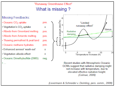
"You see most of the feedbacks are red.... But Venus?.... I don't think it will ever happen, but unfortunately we have never calculated this. It can't be done with state of the art GCMs of course. But we are thinking in Potsdam about doing first conceptual models about it.... Just to open up this field".
    0 0
  28. David, Hansen's argument for why a runaway might occur is extremely unconvincing, nor do I really think he understands how a runaway greenhouse operates. The physics outlined in this post rules out a water vapor runaway because there simply isn't enough sunlight to sustain such a situation, as has also been outlined in a number of articles on the subject (see some older papers by James Kasting for example, or Selsis et al 2007, as well as Ray Pierrehumbert's new climate book). Clouds could, in principle, change that argument but if the Earth were relatively prone to a runaway greenhouse effect, it is very likely it would have occurred in many hothouse climates of the distant past, even with a slightly fainter sun during many of these intervals. Even CO2/CH4 feedbacks don't fundamentally alter that picture, because in the runaway limit the OLR is determined primarily by water vapor and clouds. That said, the fact that a runaway greenhouse couldn't occur is really a distraction from the point that climate sensitivity could be 3 or 4 C per doubling of CO2 (or even higher on longer timescales), and we are more than capable of tripling or quadrupling CO2 levels.
    0 0
  29. A positive feed back can also be limited by the cause running out. For instance, if all the methane of the Arctic permafrost rapidly enters the atmosphere due to the observed warming of high latitudes, this will cause a run away green house effect until it is all used up. Over a few decades, the methane will oxidize to Carbon dioxide which will reduce its effect. We could see some severe bounces in temperature which then decrease to a higher level than before the bounce. I wonder how many of us will be around following such a rapid change in our climate.
    0 0
  30. Point 1: I agree with sauerj#16 that more can be done to extend this article, eg, by looking at how H2O affects climate sensitivity all else remaining equal. It's not clear to many that H2O is a dominant effect that has only kicked in aggressively for temperatures in the vicinity of where we are (eg, say within the last 10 K, I'd guess). Of the 33 ghg warming, a major contributions is only "now" being added, because of H2O. In other words, the *average* sensitivity of the planet (eg, starting from no sun or from 1.0 albedo) is much lower than the current sensitivity. We note this by looking at instantaneous tangent line slope (derivative) vs the secant that represents the average slope between our current point and the origin. I started writing up something very similar (but instead TOA flux vs surface flux), as I think showing that graph would help commentator "RW" clear remaining doubts. Ie, it would explain what sensitivity is and how it grows much faster as H2O vapor grows appreciably for a given level of CO2; all other ghg gases remaining constant, add heat from the sun has a much more powerful effect once H2O kicks in past the level needed to match the other ghg effects (earth generally has existed in that range thanks to its distance from the sun, etc). Also, I would place temp on the y axis in order to make it easier for those with modest mathematical bent to follow. You want agreement with the climate sensitivity definition if possible. Greater climate sensitivity should be seen as greater slope on the curve (in the traditional mathematical sense of y_delta/x_delta) and not a smaller/flatter slope. The sensitivity question is a very important one and should be highlighted well.. Point 2: However, I would consider an article view (or related article) to appeal to engineers [can skepticalscience add an "engineer view" for select articles.. beyond the easy, intermediate, advanced views?]. I would clarify that "positive feedback", as it is used in system's analysis and various engineering disciplines, has a different definition than climate positive feedback. This article covered the essence of this point (runaway vs not runaway), of course, but more can be said explicitly to place it in the context of traditional "positive feedback". I have noted that many engineers are skeptic, and I can relate to this particular misunderstanding. So, what describes the earth system is "negative feedback" (in the engineering sense) with a small amplitude component that likely is positive but some skeptic scientists claim could be negative due to clouds. Climate scientists don't expect that positive component to be larger in magnitude than the base negative feedback (at least not any time soon and/or within the confines of existing parameters). The key point is that any net (engineering) "positive feedback" leads to runaway behavior, by the definition used by many engineers, and we want to clarify this issue. It should be clarified that climate scientists call positive feedback simply a less negative feedback. Also, the climate models aren't feedback models, so this distinction is not important for generating future projections. In other words, the scientists' "mislabeling" is inconsequential to the calculations they perform. The "negative feedback" (engineering definition) of climate models is implicit (as mentioned in this article) from the obvious cooling effect of the 0 Kelvin outer space boundary condition and how that is incorporated into the calculations. I will look more carefully at Lindzen's "tropics" feedback analysis (maybe others have already) to see if this issue crops up. It probably isn't an issue, but I am curious. Point 3: I suspect that the albedo might change significantly if ice cover starts to disappear in very large amounts. I might not be thinking clearly, but a change in albedo of say 20% (eg, .06) would be more than merely Apocalyptic when we consider how little the earth's effective emissivity to shortwave changes with a few degrees C change at the surface (right?). Isn't most natural variability equivalent to say +/- .5 C, and isn't this change associated with a tiny percentage change in solar irradiance? Now imagine an increase of 20% incident solar flux rather than a fraction of 1%. [Am I missing something?] [BTW, I am fairly new to this and have lots to learn so I might have misjudged various issues here.]
    0 0
  31. Chris, [snipped] Your participation in discussions relating to radiative processes at the "Science of Doom" was stimulating even though we seldom agreed. Here is a question for you. I am a physicist. Other physicists such as Nikolov and Zeller and Robert G. Brown can explain planetary surface temperatures based on TSI, Stephan-Boltzman, albedos and the gas laws. So why do you think that Radiative Transfer Equations (RTEs) have any significant influence?
    0 0
  32. > It's not clear to many that H2O is a dominant effect that has only kicked in aggressively for temperatures in the vicinity of where we are (eg, say within the last 10 K, I'd guess) First of all, I am not clear on this since I have not thought about it for too long and haven't come across the statement above. Second, would I be guessing well by saying that, instead of "10K" (a mistake), 20-30K lower in global average temp would result in non-dominating ghg effect contributions from H2O and the correspondingly lower climate sensitivity, as judging by this graph http://upload.wikimedia.org/wikipedia/commons/4/41/Relative_Humidity.png and considering that H2O is about 70% of the ghg effect today with CO2 making up the majority of the rest?
    0 0
  33. gallopingcamel - I have two issues with your last post: (1) No links. No references. (2) No assertions or evidence from those authors to be considered. What is it that you are asking?
    0 0
  34. Jose X, thanks for your comments. Your understanding is rather good for being new, but just to reply to a few issues: 1) It's certainly true that climate sensitivity is a function of the equilibrium climate, and to what extent it can be linearized for small changes is still up for some debate. This is one of the issues with using paleoclimate data from the Last Glacial Maximum and applying it to the future. But I wouldn't put much meaning into the "average sensitivity" of the planet. Radiative transfer is a rather non-linear subject, and a lot of people run into mistakes of trying to figure out the sensitivity of a doubling of CO2, from say, how much CO2 contributes to the 33 K greenhouse effect. By the way, I guess I should have specified, but the outgoing radiation in these plots is all from TOA, not surface. Also, climate sensitivity is frequently taken as being inversely related to the slope of TOA flux vs. surface temperatures (e.g., see this graphic) 2) Your point about varying definitions of 'feedback' are well taken. Lindzen does describe the theory of some of this well in several of his papers, but I think one of the most definitive sources is Roe, 2009. 3) Your point 3 is off-target because ice on Earth is only a very small contribution to the planetary albedo (which is dominated by clouds, whose distribution is governed largely by the large-scale dynamics). Ice albedo is important as a local feedback, and there would be a lot of climate consequences to melting the ice (sea level, altering the atmospheric circulation, etc) but it wouldn't have the type of impact on albedo that you're talking about.
    0 0
  35. gallopingcamel, These exchanges really take away from interesting science, and your claims have absolutely no merit. I'd ask that you read an intro radiation textbook (see Grant Petty for a good undergrad level text that is still quantitative and sophisticated enough for solid understanding).
    0 0
  36. Chris #25, I agree Charlie is correct, but I think you are misunderstanding something. It's not the amplitude of that expression you mentioned that defined pos/neg in the traditional feedback sense since the sign is not changing in that expression (only the magnitude). Net negative feedback from Stefan-B (as Charlie mentioned) means that as we increase temperature we get a counter effect to that raise (a dampening effect.. a "force" that would otherwise make T decrease if it could exist by itself). If we had net positive feedback (in the traditional/engineering sense), on the other hand, we'd get a runaway effect such as one sees when a microphone is brought too close to the speakers.. the signal amplitude blows up very fast (until saturation is hit or some circuit is tripped and shuts it off). Of course, the earth never gets rid of the S-B radiation loss into space, so any "positive feedback" claims would be impossible except within the context of a limited model range (eg, the mic/speaker goes through runaway but only until saturation where the model goes beyond its capabilities... obviously, the mic/speaker runaway doesn't turn into a black hole and suck all the energy from the universe). As stated in Jose_X #30, I do think clarifying well how climate positive feedback is not the same thing at all as traditional (engineering) positive feedback would really get a lot more engineers to pay attention and say "oh, that's what they mean". The climate scientists appear to be in an imaginary world to some engineers first looking at this question of pos vs neg climate feedback. Just like you think Hansen is off, many engineers think all of climate science must likely be off in thinking we are *currently* in a runaway situation that will inevitably consume the entire planet. Perhaps those climate scientists don't even know mathematics. Someone has been conning them to use some computer program and they blissfully live in their own made-up world. [In reality, many engineers probably suspect they are misunderstanding something, but the net result is similar if instead of learning and becoming advocates they lose interest and perhaps afterward sign on to some Internet list of skeptics.] Feedback analysis obviously has limitations. I would not criticize the definitions used in climate science since those appear to be useful definitions for the context, but, I think this change in definitions should be made more clear to an audience composed of technically savvy people. I would consider adding in an "argument" on the website that addresses this feedback issue, even if the audience would be limited. The educated engineer/scientist(?) is an influential audience and can be quiet a thorn or otherwise a useful ally.
    0 0
  37. Chris #34, >> But I wouldn't put much meaning into the "average sensitivity" of the planet. .. a lot of people run into mistakes of trying to figure out the sensitivity of a doubling of CO2, from say, how much CO2 contributes to the 33 K greenhouse effect. Exactly. I think this is something that at least some people might not realize. Since I have seen RW's comments on various forums, I not only think this is/was a main issue s/he did not see, but many of the people replying to RW apparently didn't clearly understand this was the problem. The responses did almost inevitably include someone early on pointing out the non-linearity issue, but possibly RW did not realize what that meant and then the conversation moved on to different argumentation. A graph can help people understand that point. Mind you, I haven't seen too many people get hung up on that (certainly not like RW), but the doubt might be lingering without them being able to put it into words. Look at the reaction of sauerj#16 to a related issue.. cleared up by this very nice presentation. Additionally, showing a nonlinear curve that shows H2O effect kicking in gives insight that it's not really CO2 that does the damage. Seeing a graph with the increased (or decreased) slope and a bit of a "knee bend" (when seen from afar.. to see the forest from the trees) helps add urgency and legitimacy to the fears of many climate scientists. >> climate sensitivity is frequently taken as being inversely related to the slope of TOA flux vs. surface temperatures Thanks for the heads up. It still might be interesting to consider the flipped graph since a higher slope is probably more closely associated in the mind with a threat in most uses. A logarithm, for example, is more likely to be seen as "safe" than an exponential curve[*]. This is perhaps another case where those new to the field are likely to misinterpret. Most people's experience (of those who remember) is that we vary the x coordinate to see the effect in the y coordinate. y=f(x). More people might better understand, if you are varying a forcing[**] to then examine the effect on temperature, that you are varying the x coordinate to measure a change in the y. This view is more intuitive probably to most thinking cause-effect relationship. [*] Note, that the main topic being tossed around by laypeople is this "climate sensitivity" value, so it might help to see that relationship directly on a graph as we might be likely to interpret that graph ("cause-effect" <-> "x-y"). [**] "Forcing" is another term that I recently saw clarified that might confuse some people when hearing "CO2 forcing". As concerns the feedback confusion, engineers would likely model CO2 within the system equations. Someone recently wrote somewhere that it's equivalent to knobs being turned in a sound processing unit.. You don't model that as adding a signal strength but rather by varying parameters of the system. Eg, you wouldn't add a force vector but you'd change a viscosity coefficient. Writing an article to explain why 2xCO2 is modeled as a forcing (for sensitivity analysis) could help. >> I think one of the most definitive sources is Roe, 2009. Thanks, I had just downloaded that this week (from a judithcurry link I saved, where she too recommended it). A shorter more accessible description (and on this site) than a 25-page pdf that a friend might point towards might increase the number of people who read that. [I'll go and read it soon I suppose.] >> ice on Earth is only a very small contribution to the planetary albedo I did not realize that. Maybe here too is a lesson of sorts since I probably developed that intuition from comments made by others and from the idea that rays bouncing off the earth makes sense off a white surface. I know that the incident angle plays a much greater role, but I still got the impression ice was significant (although it is at the poles mainly, meaning there is less contribution to average albedo as the incident angle effect already probably dominates).
    0 0
  38. Jose_X #36 >Chris #25, I meant Chris #24. Also, thanks for that explanation in #24 since I had seen that equation recently but it had turned me off from reading too much more (of whatever it is I was reading related to feedbacks).
    0 0
  39. GC - do any of these theories you mention include predicting the lapse rate (ie these are not variations on Postma's stuff. And also manage to explain the observed DLR somehow does not cause surface temperature to increase? A link to a full, mathematical exposition (preferably published) would be appreciated.
    0 0
  40. Chris @35. Thanks for recommending Grant & Petty but you are a little late. In the same spirit may I recommend you read Rodrigo Caballero (University College, Dublin): http://maths.ucd.ie/met/msc/PhysMet/PhysMetLectNotes.pdf scaddenp @35, The N&K calculations I was referring to in #31 are based on physical laws from which the DALR can be derived. One of the quibbles I have with N&K is that their calculations do not make corrections for water vapor (moist adiabat). Even so, their analysis fits the facts very well for Earth, Venus and Titan: http://wattsupwiththat.com/2011/12/29/unified-theory-of-climate/ In a nutshell, the main variables that determine planetary surface temperatures are TSI (Total Solar Irradiance), and surface pressure). There are plenty of smaller influences such as albedo, cloud cover, ocean currents etc. There are even some respected scientists who claim that CO2 affects the climate. For example, Richard Lindzen: http://judithcurry.com/2012/02/27/lindzens-seminar-at-the-house-of-commons/#more-7386
    0 0
  41. Some important differences I have noticed between what I remember (or looked up) from feedback analysis and what I see in Roe2009: When system subblocks are analyzed, a transfer function is considered. Transfer functions may be the result of Fourier Transforms. These transfer functions will have dependencies on frequency. This frequency domain approach allows time domain convolusions (which are necessary calculations to understand system response to inputs) to be replaced with simple multiplication of the system functions. Further, the subblocks tend to be attached to each other through some sort of nonlinear mechanism that allows two signals from two or more subblocks to unite or to multiply with negligible coupling (eg, opamps for analog modules; standard digital circuits mechanisms; nonlinear nonmodeled mechanisms (possibly using electronics as control) between physical nonelectronic components)). This isolation is implicit in this modeling leveraging transfer functions. OK, so Roe2009 doesn't really apply these items just mentioned. The climate doesn't readily appear to have these nonlinear buffer zones that would allow subblock transfer functions to multiply as depicted on page 5, for example. I'm only on page 6, but I have seen no invocation of Fourier or other transforms to derive such transfer functions. Pictorially, there is no traditional "+" or "-" uniting the feedback path to the main one or to any other path, bringing doubt to this idea of isolation between subblocks. The 2xCO2 forcing appears to be a monotonically increasing function of some sort or at least an almost acyclical or perhaps very low frequency signal (relative to important system time constants.. I'm guessing). And of course, the principal negative feedback (S-B radiation/cooling) is not modeled as a feedback. In short, I don't question (or for that matter ascertain) the accuracy of the sensitivity analysis in Roe2009 from what I have seen so far (mostly through page 6 of 25), but it doesn't resemble at all the "feedback analysis" that I am familiar with from engineering, even though the language used in Roe2009 and many of the features of the analysis appear to mimic traditional feedback analysis. [At least based on my modest/low level of experience.] Interesting. I have much to think about and read. Any insight into this would be appreciated.
    0 0
  42. gallopingcamel #40, we should have a conversation on that WUWT article over there not here; but what I saw when I glanced at it just now were a few mathematical claims (which I have not yet verified but which conclusions seems inaccurate) made on what is recognized to be a simplified radiation model (that everyone knows doesn't include convection or high precision radiation absorption and so is used as a toy for introductory purposes) purporting to dispel the foundation of climate science. This makes no sense obviously (read between parenthesis above). Then they suggest a theory that appears to be curve fitting with little or no derivation from first principles. To recap: they attack the wrong model, probably making mathematical mistakes somewhere, and then put up a "theory" that is but a formula they hatched out by looking at data points. What kind of predictive capabilities can we expect from a formula based on curve fitting today's earth data points and no understanding of the dynamics of our changing planet? [That was a rhetorical question, but I'll answer it: probably little better than what trend analysis predictions offers us on distant future stock market behavior. Next to nada.] I think this comment is off topic, but I couldn't help myself.
    0 0
  43. It is always amazing to see how many radical paradigm shifts occur at WUWT and yet never get published, appear in any textbooks, or get discussed by the broader community. If WUWT were always right, essentially all sub-disciplines of climate, planetary science, astronomy, etc would need radical revision. Now since most have us have grown up to feel the need to glorify everyone's pet theory and opinions, and that many have a "Galileo" interpretation of how science generally advances, I suspect it won't be good enough to ask people to think about the above paragraph and have some self-skepticism. I also doubt it would be good enough to ask people who believe that sort of stuff to go buy a thermodynamics and radiation textbook, because I'm quite confident they have no interest. Of course, everyone at WUWT have bought into the argument as the deathbed of AGW, just like every other post they out up there, even if those other posts completely contradict that idea (such as Lindzen's post, which recognizes the existence of a greenhouse effect, but thinks sensitivity is very low). The only reasonable comments I've seen on that thread are from Joel Shore, who also co-authored the rebuttal (wuth me, and others) the Gerlich and Tscheuschner nonsense). I defer you to his points because I don't think it's worth discussing much. Needless to say, the article does not understand why convection occurs, or how to apply the laws of thermodynamics. It sort of gives the impression that none of this has been thought of before, yet it forms the foundation of basic atmospheric science and is taught in every undergrad atmospheric science department I know of.
    0 0
  44. Chris: Can you post a link to the WUWT thread you are talking about? I go there on occasion, yet seem to have missed that thread. I would like to read what arguement is the deathbed of AGW. Thank you.
    0 0
  45. So GC, as a physicist, how "skeptical" have you been of this unpublished work? And how do you reconcile it with say the standard physics of Grant & Petty?
    0 0
  46. Camburn - it is GC's link unified theory of climate. Spenser has take on it by the way too - see his 30 Dec 2011 article.
    0 0
  47. Ok....I didn't miss that thread, but I didn't spend much time reading it either. Within a few paragraphs it got so silly that it wasn't worth wasting time on. Somehow, I don't think the Unified Theory of Climate is the deathbed of AGW. I could be wrong, but if I am I promise that I will buy back that bridge I am now offering to anyone who believes this theory. In fact, I will even buy it back at twice the purchase price. And this is one inexpensive bridge. In fact, 100K will make a downpayment on it. Please respond to this offer via this site. IF the site slows down because of the interest in the bridge, just give it time, and I am sure your offer will make it through. Good luck on the bidding.
    0 0
  48. That WUWT thread was closed, but it does present a number of questions to simpler radiative balance models. The main problem with the article is that it claims to present a model that is better than what climate science uses but it attacks a weak model that is not used by climate science. 2.1 A) The authors fail is to ignore an assumption of the model. Their criticism is thus not accurate. The 1-shell model assumes global surface temperatures are relatively similar. This assumption is why the simple model gets ballpark figures. This assumption implies that diffusion of heat through the atmosphere, wind/advection, and even side-to-side radiation together are highly efficient and help preserve the temperature everywhere on earth within a very "narrow" range. Because of this assumption implicit in the model, convection and 3D radiation need not be modeled explicitly, but their existence is leveraged as it is clearly a requirement for justifying using S/4. While observed temperatures around the world are not all even, these assumptions appear to be acceptable to first approximation. Note that clearly no significant chunk of earth's surface air temperature is near 0 K or near 120 C, the two extremes based solely on sun's irradiance. So the authors ignored this assumption of the model. Were it not that the model *does* consider convection indirectly, the points raised in this section would have merit. Their math is accurate. Although, the cs constant is virtually redundant (doing little beyond adding at least 2 extra irrelevant "significant" digits to a term). Yes, it is true that if you average many temperatures near 0 K as well as a few near 100 C and everything in between (weighted largely towards the low values), you get something rather different and significantly lower than the actual average. [I spent some time making sure the integral was set up properly (that the error from the strips making up the approximating polyhedron to the hemi-sphere did go to zero as the partition sizes got smaller). It was accurate (and I got to practice and gain insight into describing surfaces of integration). To come to that understanding, I first recognized that the outer integral with no phi dependence meant we were going around the circle adding up symmetrical "tangerine peel" slices. The d(cos (theta)) was also expanded to -sin(theta)d(theta), where theta varies from pi/2 to 0. We see that each differential (tiny) rectangle in a peel slice approaches the exact area of the underneath sphere (which looks like a flat plane). This is so because the sin (theta) factor makes sure the differential rectangles nearer to the poles are smaller exactly as dictated by the ratio of the minor circle at that latitude to the major circle at the equator (that ratio being sin(theta)/1). Since a tiny rectangle's % error goes to 0 as it gets teenier, we know the overall sum error also goes to 0 (eg, factor out the %-bounded error of each rectangle being added). With this verified, we return to d(cos (theta)) to enable a painless integration. The actual calculation is essentially K * integral (x^1/4 dx) = K*(4/5)*(x^5/4) to be evaluated from 0 to 1. Note that the dark side of the earth gets zero solar radiation, and this is accurately modeled since the integral approximating limit adds "tangerene peel" slices around only a hemisphere... yet then divides by the full surface area of the unit sphere, 4*pi.] 2.1 B) A few flaws exist in this section. First, we are adding convection to a model that already implicitly accounts for it in the lateral direction. This means that the conductance values given cannot be used since air cannot simply flow up and down at calculated linear rates while also flowing to the sides at possibly comparable rates. [Simple solution is to reduce the conductance value by 10-30%.] Second and most importantly, it fails to account for the gravitational potential energy cost of rising air, that is, for the natural equilibrium lapse rate. This mandates at least that Ta be made dependent on height (another change to the model). The simplest approach here is to set h to the height of TOA, but there are other possibilities (and emissivity would depend on height as well). Ts - Te will not be near zero but to first approx will be near the lapse rate requirements. Third, the equations solve for a steady state value. The equations are essentially devoid of a time dependency so assume S is constant. Since the earth rotates, the equilibrium values may not be reached, or at least S should be modeled as a function of time and other time dependencies should be introduced. [This point may be negligible. I haven't studied this physics, but I wanted to also list some *potential* flaws that have crossed my mind.] 2.1 C) This says very little. Keep in mind that it is criticizing what is known to be a weak radiation model. The model fails to explain the high DLR near the ground, true. One major reason for this is that H2O has a tremendous GHG effect here. A one shell model that is bound by TOA requirements obviously will fail. We would need a minimum of two shells (or a thick shell that has Te1 at the top and Te2 at the bottom). And the bottom layer would need to have an emissivity value to match the higher ghg effect of concentrated H2O. [Hottel, Leckner, and others have measured emissivity values. We can also use Beer Lambert law.]
    0 0
  49. Chris @43, During our debates on "Science of Doom", Leonard Weinstein and I pointed out that for Venus it would make little difference to the surface temperature if the CO2 were replaced by an equal mass of Argon or Helium. In case you have forgotten, here are the links: http://scienceofdoom.com/2010/06/12/venusian-mysteries/#comment-2949 http://scienceofdoom.com/2010/06/12/venusian-mysteries/#comment-2953 The DALR depends on efficient heat transfer processes. In the troposphere of rotating planets heat transport is primarily achieved through convection and baroclinic eddies (mixing). Radiative processes are important only in the stratosphere where the lapse rate is usually of the opposite sign (temperature rises with altitude). Like Weinstein and this camel, N&K conclude that gas composition has an insignificant impact on planetary surface temperatures. Observations support this idea. As this thread includes "Runaway" warming let me say that if such a thing were possible it would surely have occurred during the last billion years and we would not be having this discussion. Here is a comparison between the IPCC's models that include strong positive feedbacks with one that places more emphasis on natural processes. Please note that Scafetta is making some progress on quantifying the processes that support his model using the ACRIM satellite: http://wattsupwiththat.com/2012/01/09/scaffeta-on-his-latest-paper-harmonic-climate-model-versus-the-ipcc-general-circulation-climate-models/ I must confess to some bias as Nicola Scafetta and Robert G. Brown are members of the Duke university physics department as I was for many years. We don't always agree but they have my respect and admiration. Jose_X @48, The references I provided are from physicists who are applying thermodynamics, Stephan-Boltzman etc. To dismiss this as "curve fitting" tells me that you need to take another look at the equations.
    0 0
  50. gallopingcamel, 1: I called it curve fitting partly because I skimmed very fast on my first pass and saw very few equations. It seems the curve was fitted to data points, that it was derived through linear regression without a core physical model to justify the form and approximate values of the equations. When you derive something from more basic physical principles you leave a clear math trail that shows how the formulas led to the solution. No such trail exists was apparent, and, even if computers did much of the work of solving complex equations, I would have expected to see summarizing details of such equations. The only thing discussed significantly (that I noticed when skimming) in section 3 or 4 was pv=nrt. Even if that was at the core, you don't get the two exponential terms with very precise exponents by calling praising pv=nrt, but you can get it from a good computer program doing linear regression (which they acknowledged fit the data very well). If you want to point out to me the model/math from which their two exponential terms fall out, please do so, as it would save me time. 2: Ultimately I might be convinced that the "greenhouse effect" does not dominate. I have not derived any answers, so I don't know. I do find the greenhouse effect reasonable, and I give the benefit of the doubt that others have used computers to produced the math that separates the roles done by convection from that done by radiation (maybe this hasn't been done yet, I don't know). I don't doubt DLR and the radiation effects; however, while absorption might happen at a rate dictated by radiative theories, LTE and convection (or something else) can certainly mean that the lower gases absorb in much higher concentration than they emit. Emission can still be naturally based upon the local temperature which is regulated through some other mechanism (eg, convection) to match a natural (gravitational potential based?) lapse rate. In fact, this idea basically comes from current radiative theories (I think), except that they might not be realizing that the convection effect, when the proper physical solution is derived, dominates whatever extra absorption potential more CO2 would produce [to absorb more easily would have no effect on emission rate thanks to LTE, convection, and lapse rate tendencies, for example.]
    0 0

1  2  Next

You need to be logged in to post a comment. Login via the left margin or if you're new, register here.


The Consensus Project Website

THE ESCALATOR

(free to republish)


© Copyright 2024 John Cook
Home | Translations | About Us | Privacy | Contact Us