


 Arguments


Lessons from Past Climate Predictions: IPCC FAR
Posted on 26 August 2011 by dana1981
 The Intergovernmental Panel on Climate Change (IPCC) First Assessment Report (FAR) was published in 1990. Its purpose was to assess the available scientific information related to the various components of climate change, and to formulate realistic response strategies for the management of the climate change issue. In the process, the FAR made some projections of future global warming, whose accuracy we will evaluate in this post.
The FAR used energy balance/upwelling diffusion ocean models to estimate changes in the global-mean surface air temperature under various CO2 emissions scenarios. Details about the climate models used by the IPCC are provided in Chapter 6.6 of the report.
The IPCC FAR ran simulations using various emissions scenarios and climate models. The emissions scenarios included business as usual (BAU) and three other scenarios (B, C, D) in which global human greenhouse gas emissions began slowing in the year 2000. In 2010, the atmospheric CO2 concentration in BAU projected by the FAR was approximately 400 parts per million (ppm), and in Scenarios B, C, and D was approximately 380 ppm. In reality it was 390 ppm, so we ended up right between the various scenarios. The FAR greenhouse gas (GHG) radiative forcing and CO2-equivalent for the scenarios is shown in Figure 1.
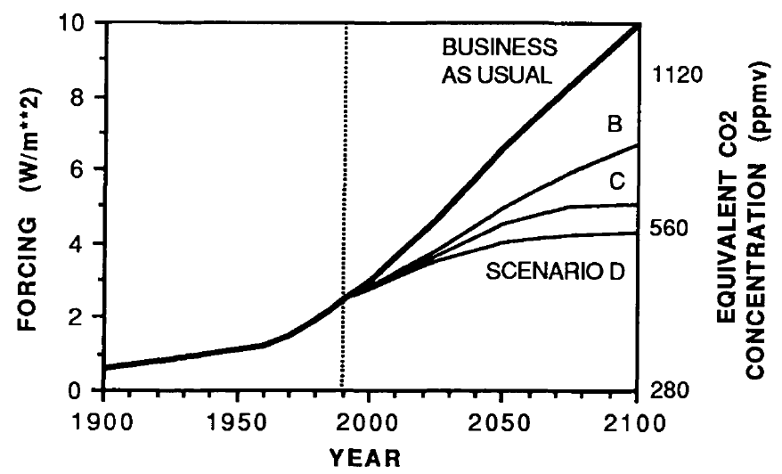
Figure 1: IPCC FAR GHG forcing and CO2-equivalent projections for the four emissions scenarios
As you can see, the FAR's projected BAU GHG radiative forcing in 2010 was approximately 3.5 Watts per square meter (W/m2). In the B, C, D scenarios, the projected 2010 forcing was nearly 3 W/m2. The actual GHG radiative forcing was approximately 2.8 W/m2, so to this point, we're actually closer to the IPCC FAR's lower emissions scenarios.
However, aerosols were a major source of uncertainty in 1990. In an improvement over Kellogg's 1979 projection study, the IPCC FAR was aware that an increase in atmospheric aerosols would cause a cooling effect. However, they had difficulty quantifying this cooling effect, and also did not know how human aerosol emissions would change in the future.
The IPCC FAR ran simulations using models with climate sensitivities of 1.5°C (low), 2.5°C (best), and 4.5°C (high) for doubled CO2 (Figure 2).
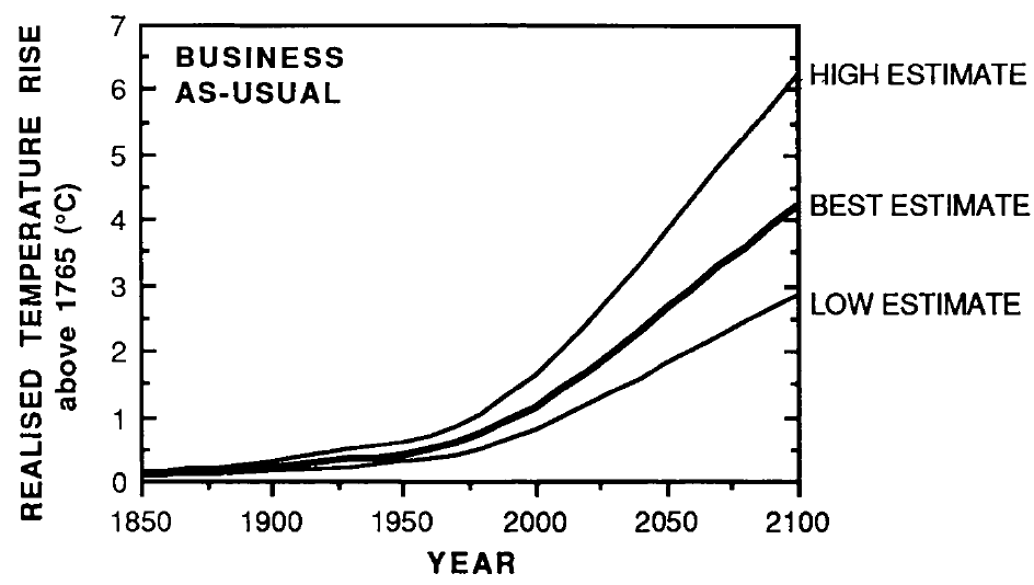
Figure 2: IPCC FAR projected global warming in the BAU emissions scenario using climate models with equilibrium climate sensitivities of 1.5°C (low), 2.5°C (best), and 4.5°C (high) for double atmospheric CO2
We digitized these projections and compared them to the observed average global surface temperature change from GISTEMP (Figure 3).
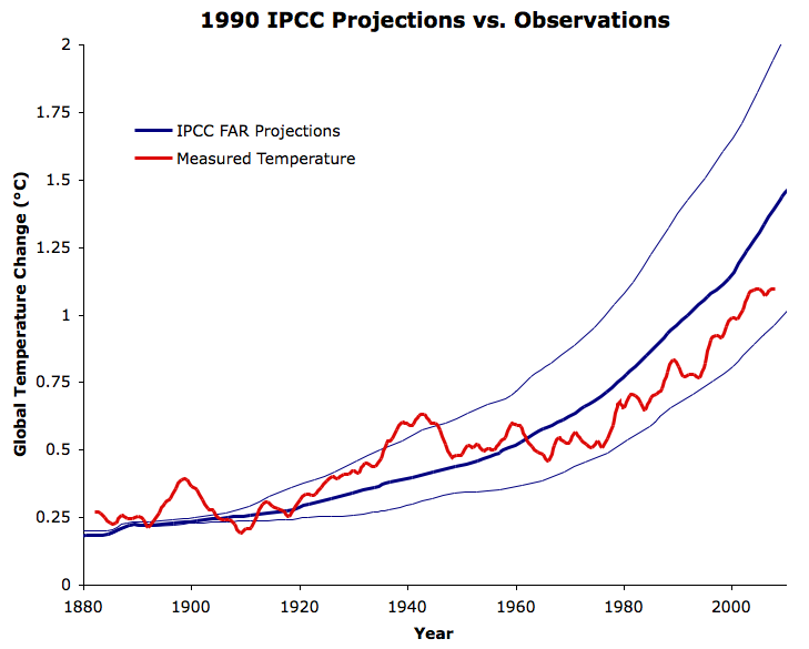
Figure 3: IPCC FAR BAU global warming projections (blue) vs. observed average global surface temperature change from GISTEMP five-year running average (red)
As you can see, the observed warming since 1880 has been between the IPCC BAU "best" (2.5°C sensitivity) and "low" (1.5°C sensitivity) projections. However, as noted above, the actual GHG increase and radiative forcing has been lower than the IPCC BAU, perhaps because of steps taken to reduce emissions like the Kyoto Protocol, or perhaps because their BAU was too pessimistic.
Regardless of the reason, we're not really interested in how well the IPCC scenarios projected the GHG changes; we want to know the accuracy of the model temperature projections. We can take the observed atmospheric GHG changes into account, and see what the model would look like with the up-to-date estimates of the GHG forcings from the 2007 IPCC Fourth Assessment Report (Figure 4).
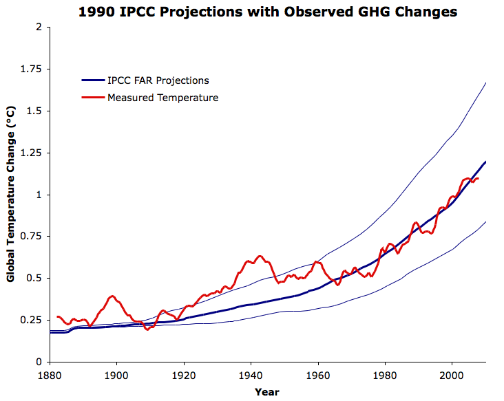
Figure 4: IPCC FAR BAU global warming projections reflecting the observed GHG changes (blue) vs. observed average global surface temperature change from GISTEMP five-year running average (red)
Obviously the IPCC model is a bit oversimplified, failing to take into account the natural factors which contributed to the pre-1940 Warming, or the factors (primarily human aerosol emissions) which contributed to the mid-century cooling. However, the IPCC "best" projection matches the long-term warming trend, particularly since about 1965, very closely. As with Broecker's 1975 prediction, this is strong evidence that human greenhouse gas emissions have been the main driver behind the observed global warming over this period, and suggests that CO2 became the dominant climate driver in the mid-20th Century.
Since the IPCC projections were made in 1990, we can also evaluate how accurately they projected the global warming over the past two decades (Figure 5).

Figure 5: IPCC FAR BAU "best" global warming projection reflecting the observed GHG changes (blue) vs. observed average global surface temperature change from GISTEMP (red) since 1990. This figure has also been added to our hi-rez graphics page.
Now we see that had the IPCC FAR correctly projected the changes in atmospheric GHG from 1990 to 2011, their "best estimate" model with a 2.5°C equilibrium climate sensitivity would have projected the ensuing global warming very accurately.
It's also important to note once again that the IPCC models did not account for changes in human aerosol emissions, which have had a significant cooling effect at least over the past decade, or natural factors like solar activity, which has declined since 1990 as well. This suggests that the IPCC "best" model equilibrium sensitivity of 2.5°C may be somewhat too low.
Accurate Climate Models
Figure 5 in particular shows once again that even two decades ago, global climate models were making very accurate projections of future global warming. As with Broecker (1975) and Hansen (1988), the accuracy of the IPCC FAR global warming projections put a dagger in the myth that models are unreliable. These results also add to the mountains of evidence that climate sensitivity is in the ballpark of 3°C for doubled atmospheric CO2.


Runrig - In the 1990 FAR report the radiative forcing from a doubling of CO2 was estimated by the equation:
ΔF = 6.3 * ln(C/C0)
In 1998 a far more extensive examination of radiative models and forcing was done (Myhre 1998), and the simplified equation (curve-fit to the radiative model results) was updated to a more accurate constant:
ΔF = 5.35 * ln(C/C0)
Constants for CH4, N2O, and CFC direct forcings were also updated in that paper. And later IPCC documents rescaled the FAR model results accordingly - entirely appropriately.
KR,
Thankyou for that.
It's what I thought - and what i told him.
He still thinks that it is "deceptive" that the IPCC in that AR5 graph has the new ECS, without reference to it's being changed.
Is that right?
There is no mention that I can see. I was hoping to pass on that statement from the IPCC to him
Tony
Runrig - I haven't dug into the history of _that particular figure_. However, the IPCC reports are of the current state of the art; the Myhre et al results were incorporated as far back as the 2001 SAR, and by now are likely just considered part of background literature/knowledge.
It's also noteworthy that the FAR projections were based on emission scenarios higher than actually occurred - I suspect some of the adjustment may come from using observed forcings to rescale FAR projections over intervening years.
Regardless, the fact that Bell hasn't come across the initial reference(s) to projection rescaling (based on forcing updates and historic emissions) shouldn't be interpreted as nefarious actions by the Illuminati, as he has apparently concluded. Rather, it means he isn't wholly familar with the literature.
Thanks again KR - If you dont mind I'll post up your response here on the Phys.org thread.
Tony
Runrig, I disagree with KR's assessment. The reason is that if you look at the IPCC FAR Chapt 6, fig 6.11, you will find it shows three panels. Panel (a) shows the high (4.5 C per doubling) climate sensitivity estimate; panel (b) shows the moderate (2.5 C per doubling) climate sensitivity estimate; and panel (c) shows the low (1.5 C per doubling) climate sensitivity estimate:
Comparing differences between 1990 and 2035, as best as I am able, the top of the range is BaU in panel (a), with an approximatley 3 C increase. In contrast, the bottom of the range (scenario D in panel (c)) shows less than 0.5 C increase. That, then, is the full range.
Now, if the climate sensitivities had been reduced inline with KR's arguments, both the top and the bottom of the range would be reduced. Instead, however, we find the top of the range shown in AR5 is 1.85C above the 1990 level, whereas the bottom of the range is 0.58 C above. Both the top of the range and the bottom of the range have been contracted towards the median value, and by about the same proportion. As a result, the bottom of the range shows a higher, not a lower value as required by KR's line of reasoning.
Even if we restrict the analysis to the median value range shown in Fig 9 of the Summary for Policy Makers, the range shown in FAR is approximately 0.6 to 1.5 C. If that is what is shown, the lower range is unadjusted (contrary to KR's explanation), and the upper range is increased.
If I were to hazard a guess as to what the IPCC has done, it would be that they have used historical values for forcings from 1990-2010, and the scenarios thereafter. If that is what they have done, it would contract both the high and low estimates towards each other as there will be less disparity in the forcing history. That, however, is only a guess, and you would have to consult with one of the IPCC authors to get a definitive answer.
Finally, I will note that if Doug Bell is going to complain about the "IPCC deception", it would behove him to show all three panels of the IPCC FAR predictions, not just the middle range values that he actually shows. That strikes me as rather more deceptive than anything the IPCC may have done. The excuse that he uses the values shown in the summary for policy makers (should he make it) is irrelevant in that the caption of the AR5 article explicitly refers to Fig 6.11 as the source of the projections shown.
Further, even using Fig 9 from the summary for policy makers, he exagerates the warming shown substantially. As noted, the difference between 1990 and 2035 for BaU in that chart is about 1.5 C. He, however, shows it as greater than 2 C.
Tom,
Thanks for the heads up on the full range of scenarios shown by AR5 ... I think the answer is therefore a simple one.
Bell is basing his analysis on the basis of just the BaU scenario ... so examining the 2 extremes of the graphs (fig 6.11), I get a range of 0.5-1.9C above '90 (+/- 0.1C) ... which is what is shown in the AR% graph!
Tony
Runrig @18, I get slightly different values, particularly for the upper range as note in my prior comment. However, given that I must judge the year by eye, and given that the reproduction of the graph shows it was a photocopy of a page, not perfectly flat on the plate, I would not argue the toss. Two points, however. First, Bell bases his analysis on the range of BaU through to scenario D on just one climate sensitivity value, rather than just BaU across the range of climate sensitivity values. Second, you mention "the full range of of scenarios". I think it is better to be more precise and mention the range of scenarios and climate sensitivities.
Tom,
thanks again - I've put the latest response from you here ...
http://phys.org/news/2015-01-climate-dont-over-predict.html
And have suggested Mr Bell call in here for more "learned" discussion.
Oh, and if you'd care to call in on Phys.org to make comments you'd be more than welcome!
Tony
I'll bow to Tom Curtis's far better researched answer on this one. :)
I just want to comment on the well thought out answers on this thread, with thanks. I should have thought to have brought the problem here, and thanks Tony for doing so.
Mr. Bell is somewhat less objective than he holds himeslf out to be. Tom. your review seems to hit the crux of the issues - Mr. Bell is using a deceptive and incomplete "analysis" as a means to call the IPCC as a whole deceptive or incompetant. I think that, in and of iteself, is enough to put his "analysis" into its proper perspective.
Thank you Tom for looking into it, and thank you Tony for bringing it here for review.
Folks,
Further to posting my/your input over at Phys.org, Mr bell posted up this (whilst not acceding defeat).
"Thank you Tony for your honest analysis and discussing the content of my claims. I'll pursue this at the discussion thread you provided.
It's too bad there aren't more people on this thread with intellectual honesty, but I do appreciate yours."
So you may well be able to take him in in person.
PS: he has been generally polite (and always with me), except when when goaded.
Tony
How do you align GISTEMP (or other data sets like HADCRUT) to a 1765 baseline?
Steyr, someone will correct me if I'm wrong, but I believe convention is that 1891-1910 is used for the pre-industrial baseline.