Climate Science Glossary

Term Lookup

Enter a term in the search box to find its definition.

Settings

Use the controls in the far right panel to increase or decrease the number of terms automatically displayed (or to completely turn that feature off).

Term Lookup

Settings


All IPCC definitions taken from Climate Change 2007: The Physical Science Basis. Working Group I Contribution to the Fourth Assessment Report of the Intergovernmental Panel on Climate Change, Annex I, Glossary, pp. 941-954. Cambridge University Press.

Home Arguments Software Resources Comments The Consensus Project Translations About Support

Twitter Facebook YouTube Mastodon MeWe

RSS Posts RSS Comments Email Subscribe


Climate's changed before
It's the sun
It's not bad
There is no consensus
It's cooling
Models are unreliable
Temp record is unreliable
Animals and plants can adapt
It hasn't warmed since 1998
Antarctica is gaining ice
View All Arguments...


Username
Password
New? Register here
Forgot your password?

Latest Posts

Archives

Patrick Michaels Continues to Distort Hansen 1988, Part 1

Posted on 24 January 2012 by dana1981

We recently examined three examples of Patrick Michaels deleting inconvenient data in his presentations of other scientists' research.  The first and most egregious of these examples occurred in 1998, when Michaels testified before Congress and deleted two of the three global warming projections from Hansen et al. (1988).  Rather than admit and apologize for this blatant distortion of the work of Hansen and colleagues, Michaels has responded by attempting to defend the indefensible.  However, his excuses for deleting Hansen's Scenarios B and C are based on erroneous assumptions as detailed below. Consequently, his presentation to Congress remains a distortion of Hansen's actual results.

radiative forcing changes 1988-1998

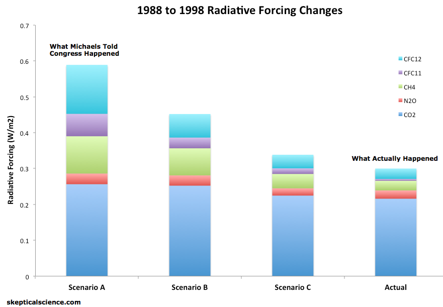
Figure 1: Radiative forcing contributions from 1988 to 1998 from CO2 (dark blue), N2O (red), CH4 (green), CFC-11 (purple), and CFC-12 (light blue) in each of the scenarios modeled in Hansen et al. 1988, vs. observations (NOAA).

Michaels' Excuses

Michaels' attempted to defend his deletion of Scenarios B and C as follows:

"I elected to focus on a comparison between the observed temperatures and those projected to have occurred under Hansen’s (in his words) “business-as-usual” (BAU) scenario."

This is the same defense Michaels put forth in 2006 when similarly accused of fraudulently misrepresenting the results of Hansen et al. in his congressional testimony.  You can read Tim Lambert's response to this defense here.

At face value, Michaels' self-defense seems like a reasonable explanation.  On the one hand, in Hansen et al. (1988), Scenario B is described as the most likely to occur (Section 4.1, Page 9345):

"Scenario B is perhaps the most plausible of the three cases"

However, in Hansen's 1988 Congressional testimony, he did describe Scenario A as "business as usual," as Michaels asserts.  But in his latest blog post, Michaels inadvertently touched upon a key point which made his testimony very, very wrong.

The Montreal Protocol

Michaels continued by describing exactly where his "BAU" assumption was false:

"Remember, this was in 1998. There was no worldwide treaty reducing carbon dioxide emissions (indeed, there isn’t one now). The only change to BAU that took place in the 1988 to 1998 time period was the Montreal Protocol limiting the emissions of CFCs."

The main difference between Hansen's emissions Scenarios A and B for the first several decades does not involve CO2.  In fact, atmospheric CO2 concentrations differ by less than 3 parts per million in 2010 between his Scenarios A and B.  No, the main difference between the scenarios involves the other greenhouse gases, primarily chlorofluorocarbons (CFCs).  In fact, CFCs account for 75% of the difference in radiative forcings from 1988 to 1998 between Scenarios A and B (see Figure 1).

In 1987, in order to address the problem of ozone depletion (also caused by CFCs), the Montreal Protocol international agreement to reduce CFC emissions was ratified, and the emissions reductions began to take effect in the 1990s.

In addition, worldwide events between 1988 and 1998, such as the collapse of the Soviet Union and tearing down of the Berlin Wall, resulted in reduced global CO2 emissions from the burning of fossil fuels.  Michaels' assumption that emissions continued on a "business as usual" path is without merit.  It should go without saying that testifying before Congress based on nothing more than unverified assumptions is generally very poor practice for any self-proclaimed expert.

Business As Usual

Michaels' entire self-defense is based on Hansen's "business as usual" comment, and his own assertion that no significant steps were taken to reduce greenhouse gas emissions between 1988 and 1998.  However, what did Hansen mean by "business as usual"?

Leading up to 1988, CFC-11 was rising at a fairly linear rate of approximately 10 parts per billion (ppb) per year, and CFC-12 by approximately 18 ppb per year.  This rate of increase is consistent with Hansen's Scenario B (see Figure 2 below).  Scenario A involved accelerating CFC emissions, so perhaps calling Scenario A "business as usual" was a poor characterization, which would be more apt for Scenario B.  In his 1988 peer-reviewed paper, Hansen had described Scenario A as (Section 4.1, Page 9345):

"Scenario A, since it is exponential, must eventually be on the high side of reality"

Perhaps a better description of Scenario A would be "worst case scenario."  Regardless, since the Montreal Protocol was implemented prior to Michaels' 1998 testimony, and other major events like the Soviet Union collapse transpired, it was not accurate for him to claim that greenhouse gas emissions had followed a "business as usual" path.  In his self-defense blog post, Michaels claimed:

"Reductions in [CFC] production began only in 1994 and the radiative effect of the Protocol by 1998 was infinitesimal."

This is simply wrong, and Michaels has not even attempted to support this false assertion.  In fact, CFC-11 and CFC-12 atmospheric concentrations only rose by 2 and 9 ppb per year from 1988 to 1998, respectively, on average.  This is a far slower rate than leading up to 1988 because of the successful implementation of the Montreal Protocol's CFC emissions phase-out.  Additionally, the other events mentioned above resulted in lower CO2 emissions between 1988 and 1998 than were modeled in either Scenario A or B; they were close to Scenario C levels.

In fact, as Figure 1 shows, the radiative forcing caused by the actual net greenhouse gas emissions from 1988 to 1998 (according to NOAA) was not only below Scenario A, but also below Scenario B, and even slightly below Scenario C.  Most of the difference was due to low CFC emissions, as well as some contribution from relatively low methane (CH4) emissions, and some contribution from low CO2 emissions.

In short, while Hansen's characterization of Scenario A as "business as usual" was arguably a poor choice, we nevertheless did not follow a business as usual emissions path between 1988 and 1998, and therefore the asserted basis of Michaels' self-defense for deleting Scenarios B and C is false.

Actual Emissions

The other major problem with Michaels' 1998 congressional testimony was in the way he presented Scenario A:

"That model predicted that global temperature between 1988 and 1997 would rise by 0.45°C...The forecast made in 1988 was an astounding failure"

This is simply a gross misrepresentation of Hansen's actual research.  First, the model did not predict temperature changes, it projected them.  The difference is a critical one.  Climate scientists cannot predict how human greenhouse gas emissions will change in the future, which is a question for the public and policymakers.  For example, we cannot expect Hansen to have predicted the Soviet Union collapse, or how successful the Montreal Protocol would be.  All climate scientists can do is project the climate effects for a given emissions scenario.

Michaels claim that Hansen's Scenario A projection was "the model prediction" was wrong.  It was one of the model predictions, based on a worst case emissions scenario which did not come to pass.

If only one of Hansen's emissions scenarios were to be presented as the model prediction, it must be the scenario most representative of actual real-world emissions. 

So which scenario was the most accurate representation?  Figure 2 below provides the answer.  The radiative forcings for Hansen's three scenarios were estimated using the simplified radiative forcing expressions from the 2001 IPCC report, based on the projected greenhouse gas atmospheric concentrations for Hansen's scenarios.  The actual radiative forcing estimates are taken from Skeie et al. (2011).

Hansen et al. only modeled the temperature response to greenhouse gas changes (and a few simulated volcanic eruptions).  So in his simulations, the GHG-only forcing and 'all forcings' are the same.  In reality, they are not, with the main non-GHG forcing involving human aerosol emissions, whose effects remain one of the biggest uncertainties in climate science.

In our analysis here, we're interested in the changes since 1988, particularly through 1998.  The radiative forcing changes since 1988 are shown in Figure 2.

Forcings since 1988

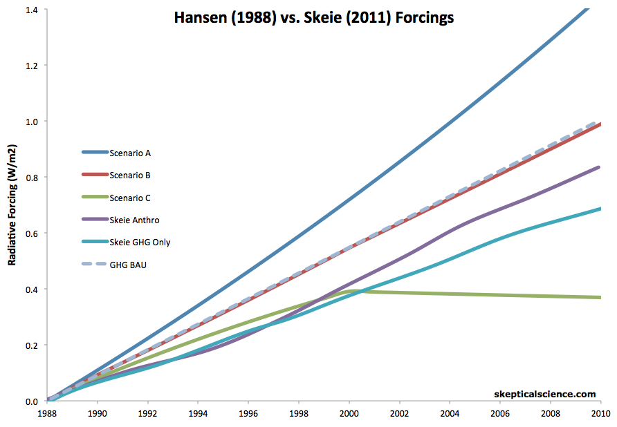
Figure 2: Radiative forcing changes (1988 to 2010) for the three emissions scenarios in Hansen et al. 1988 (dark blue [A], red [B], and green [C]) vs. Skeie et al. (2011) GHG-only (light blue) and all anthropogenic forcings (purple), and business as usual (BAU) GHG based on a rate of increase consistent with the Skeie et al. estimate for 1978 to 1988 (gray, dashed).

Both the GHG-only and net anthropogenic forcing changes between 1988 and 1998 were very close to Hansen's Scenario C, consistent with Figure 1 above, primarily due to the CFC emissions reductions as a result of the Montreal Protocol.  Business as usual GHG emissions, on the other hand, would have been on pace with Hansen's Scenario B.

In short, while Hansen was arguably wrong to call Scenario A "business as usual," Michaels' false assertion that emissions had continued on a business as usual path was (and still is) without basis, and in the process, he grossly misrepresented Hansen's research.  Michaels could easily have at least checked the Mauna Loa CO2 data to see which of Hansen's scenarios it was consistent with, but Michaels did not even do this simple check to support his false assumptions. 

Over 13 years later, even when the distortion has been pointed out many times, Michaels continues to make this false and easily debunked argument.  Before putting forth the nonsense 'BAU' argument once again, Michaels could very easily have checked the data and discovered that on average between 1979 and 1988, the GHG forcing increased 2.5% per year, versus 1.5% per year from 1988 to 1998.  Not only is this not exponential growth (as in Scenario A), but it's not even maintaining linear growth (as in Scenario B).  The data are not hard to find, so why has Michaels not even attempted to support his 'BAU' claim, and what does it say about him that he hasn't?

In Part 2, we'll examine what Michaels' presentation to Congress should have looked like, had it been accurate, and what this tells us about the accuracy of Hansen's climate model and real-world climate sensitivity.

0 0

Printable Version  |  Link to this page

Comments

Comments 1 to 27:

  1. Business-as-usual is the best description for Scenario A. There's no accuracy in calling it 'worst-case' - because it wasn't then and isn't now. Michaels' egregious distortion, a criminal act by any other name, was presenting Hanson's work to Congress with any single future line. The naming of it is minor semantics compared to the rewrite of Hansen's perspective. The alteration of removing Hanson's recognition of mega-trend variables is a disgusting smear so serious that Michaels should be held accountable for lying to Congress along the precedence set by the Barry Bonds testimony. Michaels took a strawman, and presented it to Congress as the work of James Hansen. Of course he wants the discussion to focus on the merits of his choice - so attention is diverted from his real magic trick.
    0 0
  2. owl905 @1, Hansen's scenario A was definitely a "worst case" scenario. Trivially it is the worst case of the scenarios shown. More importantly, it is, and was described by Hansen as necessarily "... on the high side of reality", at least in the long run. The later is a qualification not made by Hansen, but which I am sure he would (and would have) agreed with. Therefore, in the long run it is a worse, than worse case scenario. In the short term it is possible that worse scenarios could have occurred after 1988, but unlikely. A worse short term case would have required growth rates in GHG emissions to exceed the record levels of the 1980's, not merely retain them as is done in scenario A. Indeed, at the time of his testimony, it was known that at least some GHG emissions where likely to reduce in the near future, as the Vienna Convention for the protection of the Ozone Layer, a precursor to the Montreal Protocol, banning the use of CFC's had been negotiated, and was open to signature as of September 1987. Finally, Business As Usual is a possible descriptor of Scenario A, but only if BAU means no major economic, hiccups, and no reductions in emissions of GHG for reasons other than planned reductions to combat global warming. The first is implausible in the extreme, as we well know post Global Financial Crisis. The second was known to be probably false in 1988, not just because of the Vienna Convention, but also because the ongoing reduction of British coal mining under the control of the Conservative Party from 1984-1992. There were good reasons for Hansen to describe Scenario B as "perhaps the most plausible of the three cases" in 1988. There is certainly also good reason to consider it as the BAU scenario, although as noted, scenario A also has a claim to that title. Of course, Hansen could not anticipate the collapse of the Soviet Block, which meant that in the event, even his most optimistic scenario was on the high side of reality over the period 1988-1998.
    0 0
  3. Owl905 @1, while I obviously, and copiously disagree with your first paragraph, I want to emphasize that your second paragraph is spot on. While it is not the only issue regarding Michaels testimony and subsequent defense, it is the main issue. IMO, that Michaels testimony fraudulently presented the data is so open and shut a case, it makes a very simple test of who is guided by ideology, and who by desire for truth among so called "skeptics". If somebody cannot bring themselves to recognize that Michaels either committed scientific fraud, or at a minimum perjured himself before Congress, then there is no desire for truth in their examination of climate change issues.
    0 0
  4. @Tom Curtis - your reflection that it was a worst case, based on the expectations and outcomes of the CFC treaties, produced a guffaw'd laughter here. Kyoto stands as an example that treaties and signatures and commitments 'ain't necessarily so'. GHG emissions have been running 30% above the so-called 'worst case'. And even that's not a 'worst case', but it isn't a world away from Hansen's description of 'business as usual'. It was not, and is not, a useful description for Scenario A. Hansen's words made more sense - to frame it as a 'business-as-usual' non-response projection.
    0 0
  5. owl905 @4, while happy to cause you amusement, I suggest that your paring back a nuanced statement to just one element, thereby misrepresenting what I wrote, means you need to seriously invest in improving your reading skills.
    0 0
  6. A key point,that Hansen could not have predicted is the collapse of the USSR. Certainly this has reduced the GHG gas emissions by a large factor for at least a decade.
    0 0
  7. Indeed Yvan, the re-growth of forests in the former USSR is a major sink for atmospheric carbon dioxide too.
    0 0
  8. It should also be noted that Michaels' methodology of just taking the difference between start and end points, rather than the trend over the period, is exceedingly poor practice for anything as noisy as climate. Shift the start and end points a year or two and you can get radically different results. Obviously, this is a minor issue compared to using a data set bearing no resemblance to observations, but it is worth pointing out that he wouldn't have gotten a reliable result even if he were using the right data.
    0 0
  9. There's some subjectivity to how you define 'BAU'. To me, it's continuing on the same path as in the recent past. As Figure 2 shows, Scenario B fits that description almost perfectly. Perhaps others have a different definition of BAU. Regardless, the main point is that we did not follow a BAU path from 1988 to 1998, so the BAU definition is largely irrelevant anyway.
    0 0
  10. dana1981 @9, for me BAU means the foreseeable future development with no policies instituted to combat global warming. That may be consistent with with sharp reductions of greenhouse gas emissions if we could reasonably foresee, eg, peak oil resulting in a massive decline on fossil fuel consumption (although that consequence of peak oil, if real, is unfortunately unlikely). I can certainly see a case for calling continue current emission rates (scenario B), or continued current growth in emission rates (scenario A) as BAU.
    0 0
  11. It seems to me that the failure on Hansen's part (if it can be called a failure) to accurately define BAU is unrelated to the performance of the models. The name "business as usual" is only useful from a mitigation and prevention POV, i.e. politics, not from a predictive point of view. If we followed Scenario C closer than the others forcing-wise, then showing Scenario A (especially A) is misleading, to put it benignly. What more too, as has been shown in several previous posts, Hansen's model gave a climate sensitivity higher than the 3˚C accepted mean (4.2˚C). The model results are actually very good predictors.
    0 0
  12. @Tom Curtis - no one misrepresented your statements. My reading skills are fine. You just plain got wrong. And your ad homenem response makes a good bookend for your word-jumble to invent Hansen's response and "worst case" label.
    0 0
  13. Those who cling to the common meaning of BAU (Michaels and all his apologists) are obviously wrong. If Hansen had merely said Scenario A is BAU - and not then defined exactly what he meant by BAU - then you would have a point. But Hansen precisely defined each scenario, so the phrase/abbreviation "BAU" has no meaning whatsoever, unless it is exactly the definition Hansen provided in his paper (when evaluating his paper, not in the world at large) Another researcher, or even Michaels, is allowed to define BAU as they see fit - but no one can apply their own personal definition of BAU to Hansen's work and retain any credibility. Only Hansen's definition of BAU is valid for evaluating Hansen' work. And by Hansen's definition, we are not in BAU. That whole line of arguing is ridiculous - read any contract and you will find language which states, in the vernacular - "section headings do not supersede the precise language in each section." This is some sort of appeal to common usage which doesn't qualify as a logical error - it is just wrong - by any logical system you chose to apply. At best it is a strawman. At worst it is worthy of charges.
    0 0
  14. Dana I find the two figures confusing. It looks like actual 88-98 were below Scenario C projects. Yet we often say Hansen B is the closet to reality. And the 2nd figure doesn't seem to have all the data points that Hansen used (is that true or false?) In other words, is Skeie GHG only what Hansen was counting? (which would support B) Whose definition of GHG BAU are you counting (the one that tracks Scenario B exactly?) That seems counter to Hansen's own claim that Scenario A was BAU (although I understand the "BAU" that Hansen was responding to was a geometric increase just prior to his paper coming out). thanks to anyone who can shed light on this
    0 0
  15. actually thoughtful @14 - Scenario C was closest to reality in 1998. Currently, Scenario B is closest to reality. Scenario B is arguably closest to 'business as usual', depending on how you define the term. My definition of BAU is continuing with the same rate of emissions as in previous years. The BAU dashed line in Figure 2 is extrapolates the 1978-1988 emissions rate forward (in other words, if emissions after 1988 continued to rise at the same rate as they had from 1978-1988). See the figure caption.
    0 0
  16. There's also the question as to whether we should be comparing Hansen's scenarios to the GHG-only forcing or the net forcing. I think there are two different answers, depending on the situation: If you want to evaluate the temperature response (as we'll do in Part 2), then you should look at the net forcing. This is because the model temperature response prediction is based on the total net forcing. It just so happens that the only forcings input into Hansen's model are GHGs (and a couple volcanic eruption simulations). If you want to evaluate whether we're on a 'BAU' path based on my definition in comment #15, then you should compare Hansen's to the GHG-only forcing. This is because Hansen's definition of 'BAU' only included GHGs, not aerosols or land use changes or other forcings. Michaels' definition of BAU also only examines GHGs. That's why I plotted GHG-only as BAU in Figure 2.
    0 0
  17. actually thoughtful @14: Comparing the Scenario results raw to temperature data isn't exactly the best thing to do because the models are erroneous in two regards. The first doesn't have to do with the models, but instead with the input - too high of assumed future greenhouse gas concentrations, and the lack of aerosol forcing. The net forcing for Scenario B is higher than reality, so the model will predict a higher temperature due to that. The second reason is that the model gives a climate sensitivity of 4.2˚C/2xCO2, which is higher than the accepted mean of 3.0˚C. These issues are better explained in the rebuttal to the "Hansen is wrong" myth.
    0 0
  18. We're also going to address the climate model sensitivity in Part 2 tomorrow.
    0 0
  19. Ale and Dana - thanks to you both - I am getting a handle on it. I understand the 4.2 vs 3.0, and that aerosols were a cooling factor not completely understood in 1988. It seems, in a sense, that Hansen got lucky in that he overestimated sensitivity and ignored aerosols, and those two were of roughly the same magnitude (no disrespect to Hansen about luck - I understand one earns luck through hard work). I will read tomorrow's and see if that doesn't fill in the missing pieces for me.
    0 0
  20. About projections and models. Long lived CFC’s, Methane, Nitrous Oxide uptake and the destruction of the northern hemisphere Ozone Layer The ozone hole which appeared in 2011, 220dobson was predicted by Shindell et al in 1998 to occur 2010-2019. Now with all the other Greenhouse gases and BAU++ scenarios we are on, the ozone layer's future is at peril.
    0 0
  21. Hank Roberts at Eli's place nicely summarizes what Pat and Chip are doing: "Hank Roberts said... You have to remember he does _advocacy_. "the natural conclusion to be drawn from the omission of a fact is that the fact did not occur." Modern trial advocacy: analysis and practice -- By Steven Lubet"
    0 0
  22. Reading that CO2 increase has not been exponential in the Michaels rebuttals here over the past week or so, I had this nagging memory that Tamino had come up with a different conclusion, so today I checked back.
    "Over time, the growth of CO2 has NOT been linear, but it also has NOT been exponential. It’s been faster than exponential (as the logarithm has grown faster-than-linear, i.e., it has accelerated). And yes, the acceleration of log(CO2) (the faster-than-exponential growth of CO2) is statistically significant... ... Note that the rate is increasing overall, it’s even increasing recently; the last 10-year interval has a higher growth rate than the 1-year-preceding interval."
    http://tamino.wordpress.com/2010/04/12/monckey-business/ He says the same in a follow-up post. http://tamino.wordpress.com/2010/08/09/mo-better-monckey-business/ Tamino doesn't examine the exact period under discussion here. Is it that the trend in CO2 accumulation for the specific period Michaels examined is NOT exponential, where it IS exponential in longer time periods and/or in more recent times? It would seem so eyeballing the graphs hither and thither, but it would be nice to have that confirmed by someone with skillz.
    0 0
  23. Barry @22, "Is it that the trend in CO2 accumulation for the specific period Michaels examined is NOT exponential, where it IS exponential in longer time periods and/or in more recent times?" In short yes, the "faster than exponential" applies when one look sat the entire Mauna Loa time series-- at least as far as I can tell. But to the issue at hand. The graph below that Tamino generated represents the "linear regression slope for 10-year intervals with start times spaced 1 year apart". So the rate in 1998 is the rate over the preceding ten years. Note what happens between 1988 and 1998-- there is marked dip with the decadal rate started to decrease in 1983-1993 with the minimum decadal rate observed for 1988-1998. [Source] What happened between 1988 and 1998 was not BAU as Michaels claimed-- Michaels was flat out wrong.
    0 0
  24. For any readers who are unsure of the maths, a linear growth rate is a constant absolute growth rate in absolute termw, while an exponential growth rate means a constant percentage growth rate. With variable growth percentages, we take the geometric mean to determine the constant growth rate over a period that would have resulted in the same growth rate. Having done so, we find that the geometric mean of the growth rate in CO2 concentrations from 1978-1987 was 0.436%, while that from 1998-2007 was 0.515%, a clear increase, or more than exponential growth. In contrast, the geometric mean of the growth rate over the period 1988-1997, the period covered by Michaels' testimony, was 0.387%, a clear decline from the previous decade, and hence less than exponential growth. Indeed, as Albatross's graph shows above, for much of that decade, CO2 levels did not even maintain linear growth. For what it is worth, the geometric mean of growth rates in CO2 over the period 1988-97 in Hansen's scenarios are: Scenario A: 0.475% Scenario B: 0.470% Scenario C: 0.422% In other words, the growth rate in CO2 concentration over the period covered by Michaels testimony was two thirds as much below that in Scenario C ( 0.035%) as Scenario A was above Scenario C (0.053%), and seventeen times as much below Scenario B (0.087%) as scenario A was above Scenario B (0.005%). On that basis, apparently, Michaels concluded that scenario A GHG concentrations matched reality sufficiently better than Scenario B or C that the latter two could be excluded without comment.
    0 0
  25. Thanks, Albatross.
    0 0
  26. I think the best way to look at Hansen 1988 is if emission a are A, then the result is A' If the emissions are B then ----- etc.
    0 0
  27. bibasir @26, exactly correct. Of course, over the period of interest, emissions were less than Scenario C. That explains exactly why Michaels only reported Scenario A.
    0 0

You need to be logged in to post a comment. Login via the left margin or if you're new, register here.


The Consensus Project Website

THE ESCALATOR

(free to republish)


© Copyright 2024 John Cook
Home | Translations | About Us | Privacy | Contact Us