


 Arguments


Recent Comments
Prev 901 902 903 904 905 906 907 908 909 910 911 912 913 914 915 916 Next
Comments 45401 to 45450:
-
R. Gates at 04:43 AM on 16 May 2013Another Piece of the Global Warming Puzzle - More Efficient Ocean Heat Uptake
Rob,
I completely agree with you about SST's as a poor diagnostic tool for global warming. They really just tell more about the energy leaving the ocean to the atmosphere. After the 97-98 El Nino with such high SST's, it would be more accurate to have said "look how much heat WAS in the ocean", rather than "look how much the oceans are warming."
I think overall we are saying the same thing about ocean heat storage and simply differ on perspective. You say the oceans are getting better at heat uptake, and I look at it as they are not passing as much back to the atmosphere-- but the net result is exactly the same in that much of the measured TOA imbalance can be found in the oceans, albeit we need a lot more data below 2000 meters.
Incendentally, here's some independent research that seems to confirm ocean warming over the past 40 years, showing that despite the uncertainties and calibration issues, even the older XBT data was accurate at showing the upward trend:
http://phys.org/news/2013-05-fish-thermometer-reveals-long-standing-global.html
-
Dikran Marsupial at 04:38 AM on 16 May 2013The anthropogenic global warming rate: Is it steady for the last 100 years? Part 2.
From Page 595 of the IPCC AR4:
8.1.2.3 Testing Models Against Past and Present Climate
...
Differences between model and observations should be
considered insignificant if they are within:- unpredictable internal variability (e.g., the observational period contained an unusual number of El Niño events);
- expected differences in forcing (e.g., observations for the 1990s compared with a ‘pre-industrial’ model control run); or
- uncertainties in the observed fields.
Note in particular, item 1. If someone wants to show that the model hindcast is poor, they need to be able to show that the error exceeded the uncertainty due to internal variability.
-
heijdensejan at 03:18 AM on 16 May 2013The last time carbon dioxide concentrations were around 400ppm: a snapshot from Arctic Siberia
Rob,
That's the best explanation I have heard so far! -
Dikran Marsupial at 02:17 AM on 16 May 2013The anthropogenic global warming rate: Is it steady for the last 100 years? Part 2.
On second reading, Dr Tung wrote "Compare the slope of the red curve with the slope of the black curve." They look rather similar to me, provided you aren't looking at decadal variation, which is largely due to unforced variability (e.g. ENSO) which is deliberately averaged out in computing the multi-model mean (as the "ENSO" in individual model runs can't reasonably be expected to be synchronised with the observed ENSO, as ENSO is a chaotic phenomenon).
It seems to me that the purpose of computing the multi-model mean is not well understood in discussions of climate, but the bottom line is that it is not a prediction/hindcast of the observed climate change, just a prediction/estimate of the effects of the forcing on the climate. These are not at all the same thing!
-
Dikran Marsupial at 02:11 AM on 16 May 2013The anthropogenic global warming rate: Is it steady for the last 100 years? Part 2.
Dr Tung wrote "Figure 9.5 from AR4 is the figure that I often used to show that while the warming since midcentury has been simulated quite well, the early twentieth century warming has not been simulated"
Like KR, I find this a rather odd statement. The multi-model mean is not directly a prediction/hindcast of GMST, but only of the forced component of the change in GMST. As such there is absolutely no reason to expect the observed GMST to lie any closer to the multi-model mean than within the spread of the model runs (as the spread is implicitly an estimate of the plausible magnitude of the unforced response). The figure shows that the models give as good a hindcast of 20th century temperature variations as we could reasonably expect, given what the models are actually intended to achieve.
Even if the model physics were exactly perfect, the observation would still be expected to lie only within the spread of the model runs, and there would be absolutely no reason to expect them to be any closer.
So the question I would like Dr Tung to answer is "Exactly how close to the multi-model mean would you expect the observations to lie in order to give a good hindcast of 20th century temperatures, and how would you justify this estimate of the magnitude of the unforced component?".
-
KR at 01:58 AM on 16 May 2013The anthropogenic global warming rate: Is it steady for the last 100 years? Part 2.
Dr. Tung - The comparison of models to observations show that observations are within the 2-sigma range of those models. That's not a failure of the models, but rather an indication of their success, even though the model mean averages out ENSO variations across the models.
Models that are fit to forcings and to observed ENSO variations, such as the one Kevin C pointed out, are much closer fits to the data.
---
The linear detrending of the AMO used in your paper is wholly inappropriate for attribution studies, as is noted by one of the very papers you rely on for your argument (Enfield and Cid-Serrano 2010). Forcings over the last century are non-linear, and a linear detrend leaves much of the warming signal in the AMO component, causing an underestimation of global warming as in your paper. Your assumption of linear warming is therefore a circular argument. Your cycle identification, and use of the CET, has other issues of non-periodicity as noted by Tom Curtis. And you have continued to completely ignore the energy balances (Anderson et al 2012, and for that matter Levitus et al 2001, Levitus et al 2005, and other works) that show the AMO and other internal variation cannot be contributing significantly to global warming given observed ocean heat content.
You have not, in my opinion, made your case, and I would continue to agree with the analysis first raised here - that your conclusions regarding a low warming trend are unsupported.
-
Rob Honeycutt at 01:30 AM on 16 May 2013The last time carbon dioxide concentrations were around 400ppm: a snapshot from Arctic Siberia
I've always found it interesting too. I liken it to harmonics. If you open up a piano and can sing loud enough, if you sing a D note each of the D strings in the piano will begin to vibrate symathetically. Sing a G and the G strings will vibrate.
Same thing is working, on a much smaller scale, with IR radiation. Since a CO2 molecule is configured in a way as to allow it to vibrate, it has a frequency where it will vibrate.
Sing that G note again in front of the piano. What happens when you stop? You can hear the G strings continuing to vibrate. They are "re-emitting" the note you sang.
Same thing with CO2. When it begins to vibrate in the presence of the right IR frequencies, it is "re-emitting" that same energy it absorbed.
I'm sure there's a point where the analogy breaks down but this is how I get my head around the concept.
-
Paul D at 00:03 AM on 16 May 2013The last time carbon dioxide concentrations were around 400ppm: a snapshot from Arctic Siberia
Re the Saadi Aubydi and Atomant discussion.
I actually find the concepts of distinguishing between greenhouse gases and non-greenhouse gases fascinating and I learnt a lot discovering the difference. Not just about the greenhouse effect either.
Once you get your head around the basics, you can see why molecules that are more complex than CO2 can be potent GHGs. I'm probably better at visualising what is happening than I am at understanding the maths.
-
John Mason at 23:53 PM on 15 May 2013The last time carbon dioxide concentrations were around 400ppm: a snapshot from Arctic Siberia
Thanks guys - people do come on here to learn and some of them may be genuinely inexperienced in this field of science - but we should support anybody who wants to learn - in fact I would be delighted to see more people not afraid to ask even the most basic questions.
One thing to consider is perhaps an open Q&A thread for such a purpose.....
-
Tom Curtis at 23:29 PM on 15 May 2013The last time carbon dioxide concentrations were around 400ppm: a snapshot from Arctic Siberia
Atomant @13, H2O is a greenhouse gas because the molecule has electrical poles. Specifically, the Oxygen atom atracts electrons more strongly than does the Hydrogen atom, resulting in the hydrogen atoms being positively charged when in a water molecule, with the Oxygen atom being slightly negatively charged. Further, because of the molecular configuration the water molecule has a number of vibrational modes, which makes it a strong absorber.
Of course, Hydrogen and Oxygen atoms which are neither ionized nor part of a chemical compound have no net electrical charge and cannot have no vibrational modes within the molecular bonds (which they do not have) and so do not absorbe IR light. They will absorbe light of higher frequency based on the energy levels of their electron shells.
I am glad you are so willing to go back to class on this.
-
Dikran Marsupial at 23:05 PM on 15 May 2013The last time carbon dioxide concentrations were around 400ppm: a snapshot from Arctic Siberia
@Atomant, it was a reasonable question; there is nothing to be gained by being rude and dismissive to those seeking knowledge, it does not create a good impression. See Tom's answer @ 6 for a much better approach. Skeptical science is a forum for discussing the science, which is why we generally try to adopt a calm rational tone, unlike the hyperbole and rhetoric that you tend to see in climate blogs that want to avoid discussing the science.
-
Atomant at 22:10 PM on 15 May 2013The last time carbon dioxide concentrations were around 400ppm: a snapshot from Arctic Siberia
Why CO2 is a greenhouse gas while CO and N2 are not?
Why is H2O a GHG while H and O are not? back to class.
-
Kevin C at 20:48 PM on 15 May 2013The anthropogenic global warming rate: Is it steady for the last 100 years? Part 2.
Jason: Yes, we're discussing it here.
-
Kevin C at 20:45 PM on 15 May 2013The evidence for climate change WITHOUT computer models or the IPCC
Tom: When you reduce the fitting period, the model is only fitted to observations in the fitting period (the thick part of the obs line). The R2 is based only on these observations. However having determined the parameters of the model I go back and recalculate the fitted temps using the forcings for the whole period, thus the model is extended to cover the whole period, predicting values which were not used in fitting the model. That means you can do a visual 'hold-out' test, to determine the skill of the model in predicting temperatures it has never seen.
Strictly you should also re-optimise the time coefficients of the exponentials when you do change the fit period. One day I may get round to automating this in the Javascript version.
-
Kevin C at 20:33 PM on 15 May 2013The evidence for climate change WITHOUT computer models or the IPCC
Bob: You really need about 70 years of data for the model to have any validity (i.e. change the second number but leave the first at 1880). Ideally those 70 years need a volcano and a significant change in a slower forcing. And then there are big caveats due to the uncertainty in the forcings - try double black carbon as per recent research and see what happens to TCR. So don't overinterpret this model.
However I still maintain (along with Isaac Held) that it can be a useful check on your intuition. The interesting case is comparing 1880-1997 with 1880-2011. Including the extra years increases TCR in this model. Why?
The years 1997-2011 have two features:
1. They are all much hotter than the average over the whole period.
2. There is comparatively little trend within that period.
Somewhat simplified: TCR is related to changes over a period of 70 years or so. So the trend within a 15 year period has rather little 'leverage' to affect TCR. On the other hand, the huge difference between the last 15 years and the period 70 years before, so adding more hot years at the end has a lot of 'leverge' to affect TCR.
In other words, adding more extreme hot years in a clump at the end tells us a lot more then the small variations within that clump.
-
Glenn Tamblyn at 19:15 PM on 15 May 2013Leave It in the Ground, Climate Activists Demand
Alex
Although use of FFs in farming is a small part of total FF use, it is the truely hard one to deal with. That is another reason why hitting transport and electricity generation hard and fast in a conversion to non-FFs is so important - to leave room in our allowable carbon budget for the far more essential uses in agriculture.
But not cutting FFs also constitutes a threat to agriculture as well. Yield declines due to warming are something we just can't afford. Even more worrying is what the impact of increases in climate variability. Which is worse, a 5% decline in global food yields that manifests as 6 years all at 95%, or a 5% decline that manifests as 5 years at 100% and one year at 70%? We don't have the food reserves to see us through a year of 70%. In scenario 1 we all tighten our belts. In scenario 2 10's of millions starve to death.
We are facing a food supply crisis this century due to a multitude of factors. And we are in a double bind. Act hard on FFs to address climate change and food supply comes under pressure because the supports to it are taken away. Don't act on FFs and Climate Change puts food supply under pressure.
-
JasonB at 18:41 PM on 15 May 2013The anthropogenic global warming rate: Is it steady for the last 100 years? Part 2.
That is really very cool. I'm particularly intrigued by the fact that you can actually get a very good fit for the entire series using just the years 1880-1950 (R2 = 0.714) even without the post-WWII SST corrections in the temperature data.
I'd say that "key comment from your article is overstated" is an understatement. :-)
Also intriguing is that the improvement of the qualify of the fit in the last few decades has come as a result of increasing TCR:
End Year TCR R2 2010 1.675 0.925 2000 1.603 0.881 1990 1.533 0.827 1980 1.506 0.767 1970 1.568 0.757 1960 1.490 0.747 1950 1.574 0.714 I presume that the change in TCR isn't statistically significant, due to the accuracy of the early data especially, but the fact that numerically it gets larger when we add the decade where warming supposedly "stalled" is telling...
-
Tom Curtis at 14:45 PM on 15 May 2013The anthropogenic global warming rate: Is it steady for the last 100 years? Part 2.
KK Tung @26:
1) The caption of Fig 3B of the PNAS paper (ie, the "Fig 4" above) reads:
"The CET AMO is compared with the AMO from the multiproxy data (12). The AMO Index (16) smoothed by locally weighted scatterplot smoothing (LOWESS) (19) is superimposed (in green). The LOWESS is a modified running-time mean, and its use allows the mean to extend to the beginning and end of the record. It uses quadratic fit to 25-y subintervals. It shows that the CET’s AMO agrees with the AMO Index and with the global mean after 1850 and agrees in phase with the multiproxy data in the preindustrial period."
The periods of 50 to 90 year band signal of the multiproxy data (MBH 98 RPC5) from peak to peak are approximately, 72 years, 70 years, 110 years and 76 years. There is no hint of the AMO switching to a 40 year period in the 1700s. Now, if the AMO period switched to 40 years in 1700s, and there are no 40 year cycles in the multiproxy AMO signal, they do not agree "in phase" and the appearance that they do so is only a product of your filtering. Hence, you cannot consistently claim both that the CET signal reflects the AMO in the 1700s and that MBH 98 RPC 5 is the AMO signal.
That inconsistency leaves you with a small problem. If you decide (reasonably given its low statistical significance) that MBH98 RPC 5 is not the AMO signal, then you are left struggling to explain why the AMO cannot be dectected in multi-proxy NH temperature reconstructions despite its purportedly dominating influence on NH temperatures in the twentieth century. If, instead you decide to use MBH98 RPC5 as your AMO signal, your are left struggling to explain its low variance explained and why the AMO was so uninfluential CET temperatures over much of the historical period.
2) Allowing that the AMO switched to very short periods (around 25 years in the mid 1700s), you need to explain why the AMO appears only to have high amplitudes and an extended period durring periods of significant forcing (Maunder Minimum, 20th century). Absent that explanation, the most conservative conclusion is that the extended AMO is a response to that forcing, either directly or indirectly. In that case, the AMO may complicate the timing of the response to forcing, but is not an independant factor.
3) I regard with extreme skepticism such humpty-dumpty oscillations whose periods can be stretched like taffy to suit the convenience of the theoretician. In science it is not a question of "which is to be master" but of what is observed. More specifically, the theory of the AMO is that a quasi periodic oscillation exists in the Atlantic with a period of about 65 years. Once that period can be stretched like taffy to fit any observation, you are merely defining the AMO into existence, not observing it.
4) Even if you present us with a theoretical justification for so extraordinarilly flexible an oscillation, which you have not, the mere fact of its fexibility reduces its the possibility of detecting it in that for a very flexible period (and amplitude) almost any observation can be made to fit the theory. In short, I think your theory of the AMO has become unfalsifiable and hence devoid of empirical content.
-
Tom Curtis at 14:01 PM on 15 May 2013The evidence for climate change WITHOUT computer models or the IPCC
Glenn Tamblyn @22, I used 4.57 billion years as the current age of the Sun, following Feulner 2012. That dates "about 6% weaker", ie, 94% of current luminosity, to around 0.73 billion years ago (Gya) compared to your 0.75 Gya. If Potholer was indeed referring to the Devon Island corals, the correct figure would have been about 3.8% weaker than today, but of course, those corals are not associated with the termination of a snoball Earth event.
-
KK Tung at 13:48 PM on 15 May 2013The anthropogenic global warming rate: Is it steady for the last 100 years? Part 2.
In reply to post 20 by Tom Curtis: We had discussed in our paper why we chose the band 50-90 years and exclude the band around 40 years. This was based on comparison with the global mean spectrum. We believe the 40 year oscillation, while also a part of the AMO, does not have a global manifestation. That is, it may have affected Atlantic and Europe, but not the Pacific. During the middle cycle in the 1700s 1800s, the AMO's period switched to 40 years and only part of it remained in the 50-90 year part.
No one is referring to the AMO as a sinusoidal oscillation with an unchanging amplitude and period. It is only quasi-periodic.
Moderator Response:[Sph] Date corrected as per KK Tung's later comment.
-
KK Tung at 13:38 PM on 15 May 2013The anthropogenic global warming rate: Is it steady for the last 100 years? Part 2.
In reply to post 23 by KR: Figure 9.5 from AR4 is the figure that I often used to show that while the warming since midcentury has been simulated quite well, the early twentieth century warming has not been simulated. Compare the slope of the red curve with the slope of the black curve. So far only HadGEM-ES has simulated the early twentieth century warming using forced solution by varying tropospheric aerosols, but it has other problems mentioned by zhang et al 2013.
-
mandas at 12:54 PM on 15 May 2013Schmitt and Happer manufacture doubt
The biggest shame with all of this is that I was a kid in the 60s, and grew up in wonder of the space program, and idolised all the astronauts.
And now I see that at least one of the people I idolised is - not too put to fine a point on it - a fool.
-
Glenn Tamblyn at 12:49 PM on 15 May 2013The evidence for climate change WITHOUT computer models or the IPCC
The formula for calculating the change in the Sun's Luinosity over time is
L(t) = [1+ 2/5(1-T/To)]-1 Lo
where the T is time from the birth of the sun. This will give you the luminosity change between any two points in time. The subscript 'o' is always the later of the two times. This is cited in Gough 1981, page 28
So the value you get depends on what age you use for the Earth. The standard value is 4.7 billion years. So 94% gives us 750 million years ago, 95%, 618 million years ago.
This is an increase of 40% since the birth of the Sun up to the present.
Peter does say however that it was 'around 6%'.
-
Rob Painting at 12:40 PM on 15 May 2013Another Piece of the Global Warming Puzzle - More Efficient Ocean Heat Uptake
R Gates - short-term sea surface temperatures are a poor diagnostic tool for global warming because they are strongly influenced by natural variability. A key point in Figure 1 is that very little energy is being lost from the climate system - surface temperatures are cool because of a rearrangement of heat in the ocean. During the negative phase of the Pacific Decadal Oscillation, more warming goes into the deep ocean.
If a significant portion of heat were being lost from the ocean, then it must warm surface air temperatures, before reaching the upper atmosphere and being radiated out to space. There is no way around that. That does not appear to have happened. The most likely scenario is that suggested by the climate model in Meehl (2011) & Meehl (2013) - the majority of this slowing of surface temperatures is due to natural variabilty (deep ocean warming) superimposed atop a long-term warming trend (greenhouse gas-induced warming of the surface ocean).
As for your comment about the Pacific Ocean warming, not sure what you find so perplexing about that.
-
Tom Curtis at 09:20 AM on 15 May 2013The evidence for climate change WITHOUT computer models or the IPCC
Bob @20, when I use the model, it only allows for data up to 2010. I also notice that when truncating the data from 2010 down to 1997, the Transient Climate Response (TCR) falls from 1.675 to 1.58, while the Coefficient of Determination (r2) falls from 0.925 to 0.86. The later surprises me. I also note that when the duration is reduced, the graphed observations are reduced, but the graphed model is not. I am not sure whether that is a bug or a feature.
The increase in TCR for the full 1880-2010 period is likely due to an acceleration of the underlying warmng rate due to anthropogenic factors. That is, the underlying warming is increasing faster than would be expected just from the increase in GHGs and aerosols, etc. This has been masked by a reduction in energy recieved from the Sun, along with transient effects such as ENSO and volcanoes.
-
Bob7905 at 09:01 AM on 15 May 2013The evidence for climate change WITHOUT computer models or the IPCC
Kevin C @15
I tried your model but with 1997-2011 there is a pop-up error message ("Insufficient data to fit").
Warren didn't come back but I wondered if you wouldn't mind explaining the counter-intuitive result anyway. I have always had a blind spot with statistics!
-
yphilj at 08:19 AM on 15 May 2013The last time carbon dioxide concentrations were around 400ppm: a snapshot from Arctic Siberia
Thanks Tom! Well explained.
- Phil in Colorado.
-
Tom Curtis at 08:05 AM on 15 May 2013The last time carbon dioxide concentrations were around 400ppm: a snapshot from Arctic Siberia
yphilj @11, if we were miraculously to cease all CO2 emissions today, then the natural uptake of CO2 by the ocean and biosphere would reduce the atmospheric CO2 concentration to about 310 ppmv over the next few centuries. That uptake reduction would exhaust all natural forms of CO2 uptake, so the CO2 concentration would then remain at that level for thousands of years thereafter. As it would take thousands of years to melt all the ice necessary for a 40 meter sea level rise, we would in fact expect an overall increase in temperature relative to the pre-industrial similar to that which we are currently experiencing, and a sea level rise over many centuries of several meters.
Such a miraculously rapid stop in emissions is, of course, impossible. Plausibly, with rapid action now we could stop net emissions by 2050, with a total atmospheric increase to 450 ppmv, reducing to around 325 ppmv over a few centuries. In that event, we would expect a temperature rise around 1 C over the pre-industrial with short term peaks potentially up to a degree above that. That is certainly a survivable and achievable outcome.
The risk is that we will do little or nothing, or merely stablize atmospheric CO2 levels by allowing residual emissions at a low level. In that case, we are indeed looking at 40 meter sea level rises over a millenium or so, and temperature rises that will threaten to destroy our industrial civilization, with out which the human population will crash to a billion or less.
-
yphilj at 07:39 AM on 15 May 2013The last time carbon dioxide concentrations were around 400ppm: a snapshot from Arctic Siberia
Great information, though very bad news. Does this paleo evidence imply that we are effectively locked in to 3-4 C degrees warming globally? If so, what's the logical course of action? Seemingly, even the most aggressive emission control initiatives, instantaneously put in place, would not stop the demise of civilization.
-
scaddenp at 07:21 AM on 15 May 2013Leave It in the Ground, Climate Activists Demand
Alex, I have only done the calculations for my own country (NZ) but it is heavily agriculturally based. Couple of points.
1/ the amount of energy going into agriculture is relatively small (5.2% for NZ). If that was the only thing we used FF for, then it wouldn't be problem.
2/ Providing for all current diesel use (farm and transport) could be done with biodiesel. Conventional methods would take 21% of agricultural land. However, there is a lot of work going into woody biofuel which could easily cover the requirement from marginal land instead.
3/ FF (especially petroleum) are limited. You are going to have to get off them eventually anyway. If you really need petroleum to feed 9 million people, then people are going die. It doesnt take much restriction of supply for woody biofuel to be cheaper anyway.
Remember that dealing with climate change is mostly about getting off coal. Petroleum is an incredibly useful and valuable resource and I think we are just squandering it. (Already have really).
-
KR at 04:56 AM on 15 May 2013The last time carbon dioxide concentrations were around 400ppm: a snapshot from Arctic Siberia
HJones - Not a problem; there's an amazing amount of junk including bad papers published in borderline journals floating around (such as Beck and E&E), and it's sometimes difficult to pick those out on first glance. They frequently get waved about to support bad arguments.
The appropriate and truly skeptical response to extraordinary data or conclusions is to check them out, which you did - my compliments.
-
HJones at 04:04 AM on 15 May 2013The last time carbon dioxide concentrations were around 400ppm: a snapshot from Arctic Siberia
All,
Thanks. I thought his paper was "submitted", and I assumed to be published soon. I was wrong. I thought it had a lot to do with altitude and am happy to see I was correct in that at least.
-
Tom Dayton at 03:56 AM on 15 May 2013The last time carbon dioxide concentrations were around 400ppm: a snapshot from Arctic Siberia
Saadi, one good explanation is at Science of Doom.
-
Philippe Chantreau at 03:54 AM on 15 May 2013The last time carbon dioxide concentrations were around 400ppm: a snapshot from Arctic Siberia
HJones, this horse has been beaten to death. Beck is not, and never was, a reliable source of information. The pdf you linked is not a peer-reviewed science article (it appeared in E&E but that does not qualify, sorry).
Beck's "reconstruction" is based on inaccurate methods. Furthermore, it states that there were swings in CO2 atmospheric concentration as large as 290ppm to 470ppm in 15 years. That by itself is beyond ludicrous. There is no industrial process and no known biological process that could lead to such a change in that short a time. And it's not like Beck placed this in a past devoid of humans observing the planet, it's supposed to have happened mid-20th century.
Nonetheless, let's imagine that some immense biological process took place in a totally silent way except for the CO2 fluxes. If such evens had really happened, it would have to leave an enormous C13 signature, but that is nowhere to be found. The whole thing is a pile of nonsense, it's not worth any time or attention.
-
Tom Curtis at 03:52 AM on 15 May 2013The last time carbon dioxide concentrations were around 400ppm: a snapshot from Arctic Siberia
Saadi Aubydi @3, of topic, but the short answer is that N2 and O2 are not greenhouse gases because there is no charge imbalance between the two components of the molecule. That renders the gases transparent to IR radiation. Carbon Monoxide (CO) is a weak greenhouse gas because, although it does have a charge imbalance, because it only has two molecules it is limited in the sort of vibrations it can perform, meaning it does not absorb IR radiation at the main frequencies of emission within the Earth's atmosphere. This is explained in more detail here.
-
Tom Curtis at 03:45 AM on 15 May 2013The last time carbon dioxide concentrations were around 400ppm: a snapshot from Arctic Siberia
HJones @2, the following are CO2 concentrations as measured by an aircraft in Colorado in 2004:

You will notice that while the measurements above 500 meters consistently record CO2 concentrations around 375 ppmv, those below that altitude are very variable, and much larger. That is because the CO2 concentrations below 500 meters are contaminated by local sources of CO2 (mostly forests), whereas above 500 meters the CO2 from local sources has become diluted, leaving the local concentration at the background level.
This is the problem with Beck's measurements. While accurate, they are also contaminated by local sources of emissions. Beck lumps all the measurements together without regard to whether they were taken in enclosed rooms (which can have CO2 concentrations up to 1000 ppmv with poor ventilation), in industrial cities, or in forests (which absorb CO2 in the day time, but emit it at night). He also does not distinguish between CO2 measurements in autumn (when decaying vegetation elevates local CO2 concentrations) or spring (when new growth depresses it). Because he simply ignores these relevant and well known facts, Beck's paper is propoganda, not science.
In contrast, the Mauna Loa measurements are taken at altitude away from industrial sites and forests, and only when the prevailing winds prevent contamination from the local volcano. They agree with measurements taken from many other remote sites including the South Pole.
-
KR at 03:32 AM on 15 May 2013The last time carbon dioxide concentrations were around 400ppm: a snapshot from Arctic Siberia
HJones - See the replies to Becks paper by Keeling and Meijer. Short answer: Beck made measurements at ground level, seriously contaminated by local effects, whereas the Mauna Loa (proper spelling!), Antarctic, mid-ocean, and other measures are a far more accurate background measure with care taken to avoid industrial influences. Becks methods were inappropriate, and his measurements are accordingly of little worth WRT global CO2 levels.
I suggest looking at the more accurate and widespread CO2 measures than Beck's work - it's a brief video, well worth watching.
-
Saadi Aubydi at 03:31 AM on 15 May 2013The last time carbon dioxide concentrations were around 400ppm: a snapshot from Arctic Siberia
Hi, Why CO2 is a greenhouse gas while CO and N2 are not?
-
HJones at 03:15 AM on 15 May 2013The last time carbon dioxide concentrations were around 400ppm: a snapshot from Arctic Siberia
The above link shows other values for CO2 concentrations beside Mona Lau. When did the measurements in Hawaii become the standard? Are these others even valid?
Moderator Response:[RH] Fixed link that was breaking page format.
-
John Hartz at 03:04 AM on 15 May 2013The last time carbon dioxide concentrations were around 400ppm: a snapshot from Arctic Siberia
John Mason:
Kudos on an excellent article combining a very well written text with outstanding graphics.
-
Alex in the Farmbelt at 02:06 AM on 15 May 2013Leave It in the Ground, Climate Activists Demand
I would postulate most of the carbon cycle carbon that we consume comes to us with the help of fossil fuel carbon, so it is not a zero-sum game. Tractors, irrigation motors, trucks to transport use fossil fuels and even elements of fertilizers and pesticides come from petroleum. I don't know of an electric vehicle capable of performing the work necessary to grow & distribute enough food for the masses, regardless of the source of charge. Is there a solution to nutritional needs on a scale to satisfy 7 Billion people that does not involve petroleum?
-
R. Gates at 00:21 AM on 15 May 2013Another Piece of the Global Warming Puzzle - More Efficient Ocean Heat Uptake
John Brooks,
I do not question that heat can be be advected to depths by downwelling, for certainly it can, I simply question the overall thermodynamic perspective given that the net flow of energy is always from ocean to atmosphere on a global basis. It seems more accurate to say the oceans are releasing less rather than taking up more, which is exactly the case during La Niña and cool phase PDO. In this regard, SST's are most instructive as they tell us more about heat being transferred from ocean to troposphere rather than about how much energy the ocean is storing. During the big El Niño of 1997-98, SST's were quite high, and of course that was a good indication that energy was leaving the ocean and we saw tropospheric temps rise and ocean heat content took a dive.
-
Kevin C at 23:57 PM on 14 May 2013The anthropogenic global warming rate: Is it steady for the last 100 years? Part 2.
Bart: No, it's the 2-box model of Rypdal 2012 with an extra ENSO term - the response function is determined by fitting the forced response to the data. However the forced response is similar on the decadal level to the temperatures obtained by Hansen 2011 using the Green's function mode. The only difference is that he uses the model to get the response function.
Tamino writes about his version here.
You can actually get a marginally better AIC using 1.5 boxes (1-box + transient). -
KR at 23:54 PM on 14 May 2013The anthropogenic global warming rate: Is it steady for the last 100 years? Part 2.
Dr. Tung - If you are including the aerosol forcings and their changes over time, the sum forcings are again not linear since 1910, as per the figure in my post above. Note that not only tropospheric but stratospheric aerosols are involved in the "S" curve seen in 20th century forcing data. There is simply no support for a linear forcing during the 20th century, a requirement for your claim of a linear warming since 1910.
As per Kevin Cs comment, and your claim that "no CMIP3 or CMIP5 models have successfully simulated the observed multidecadal variability in the 20th century using forced response", I would simply point out Figure 9.5 from the IPCC AR4 report:

Figure 9.5. Comparison between global mean surface temperature anomalies (°C) from observations (black) and AOGCM simulations forced with (a) both anthropogenic and natural forcings and (b) natural forcings only...
Note that the models using all forcings match multi-decadal temperature variations quite well, including a mid-century pause. I fail to see significant support for your statement.
-
Bart Verheggen at 23:43 PM on 14 May 2013The anthropogenic global warming rate: Is it steady for the last 100 years? Part 2.
Kevin, impressive comparison. Is there some more info somewhere on the ins and outs of the model and analyses used? In particular, is it using the Green's function of GISS model-E?
-
John Brookes at 23:08 PM on 14 May 2013Another Piece of the Global Warming Puzzle - More Efficient Ocean Heat Uptake
Thanks R. Gates. I had not thought of the energy flow being from the ocean to the atmosphere before, but its rather obvious now that you mention it.
-
Kevin C at 22:20 PM on 14 May 2013The anthropogenic global warming rate: Is it steady for the last 100 years? Part 2.
I think KR's comments on use of all the forcings is critical. In particular, I think that this key comment from your article is overstated:
It is fair to conclude that no CMIP3 or CMIP5 models have successfully simulated the observed multidecadal variability in the 20th century using forced response.
In fact, Hansen's model at least comes very close if you take into account internal variability in the for of El Nino. I haven't looked at the others, but here is a result from a simple 2-box model illustrating this fact:
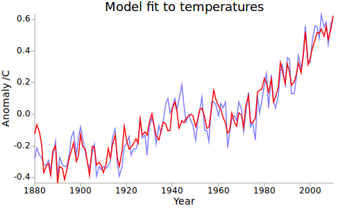
This trivially simple model is available here for you to play with - for the figure above, just click 'Calculate'.
The key to this model is that it takes into account both forced response and ENSO. If you leave out the ENSO term (figure 5 on that page), then the model appears to fail to reproduce the mid-century cooling. When including it (figure 1) the model fit is extremely good except for 2 spikes either side of WWII. The temperature record is GISTEMP and so is missing the post-war SST adjustments, which probably accounts for much of the remaining discrepancy.
The significance of the ENSO term is that the trend in MEI on the period 1940-1960 is about 70% of the trend on 1997-2013. ENSO plays a significant role in the cooling on that period, and of course only corresponds to a single realisation of climate variablility. Using an ensemble of runs or alternatively using a simple energy balance model allows us to eliminate the internal variability. Imposing the real ENSO contribution allows us to figure in the actual realisation. The resulting model fits 92% of the variance in the data. You can test the skill by omitting different periods from the model fit.
We could redo the calculation with Hansen's data instead of the 2-box model, but the results will be similar. Ideally we'd use a longer time frame too. BEST should be significantly better than CET, and the Potsdam forcing data goes back to 1800 (although I think it omits the 2nd AIE). I'm afraid I haven't had a change to do this calculation yet.
-
R. Gates at 21:48 PM on 14 May 2013Another Piece of the Global Warming Puzzle - More Efficient Ocean Heat Uptake
Rob,
Thanks for that explanation in repsonse to my post @2. It sounds plausible, but what bothers me is that the Pacific basin has not shown especially high ocean heat content increases, but rather it has been the Atlantic and Indian Ocean.
Also, @3 you said,
"There is the worrying possibility that 3 variables may have acted to slow surface warming during that time; the negative phase of the PDO, industrial sulfate pollution, and increased sulfates from increased volcanism of tropical volcanoes. Let's hope that that wasn't the case - it would imply significant surface warming when these 3 are no longer holding back greenhouse gas warming."
i think this could unfortunately be exactly the case, but I also would not discount a slight downward nudge from our rather sleepy sun during that time as well-- meaning that could even be a fourth factor. We had some very low total solar irradiance, and of course a current solar cycle that is the weakest in a century.
-
Rob Painting at 21:38 PM on 14 May 20132013 SkS Weekly Digest #19
Seahuck - Not a good piece by Gillis. Relatively easy adaptation to climate change is simply a fantasy. Last time I checked, ocean acidification is still happening, and coral reefs the world over are in dramatic decline. Once the reefs and productive fisheries collapse (which they are on course to), I don't expect adaptation will be an apt description of what follows.
-
Tom Curtis at 19:16 PM on 14 May 2013The anthropogenic global warming rate: Is it steady for the last 100 years? Part 2.
KK Tung @16, here are the 10, 15 and 20 year running means of the CET from 1660 to 2012:

As you can see, there is no consistent 50-80 year oscilation in the data. There is what might be a large amplitude 80 year oscillation from 1660-1740. However, the trough of that "cycle" corresponds with the Maunder Minimum and a large number of large volcanic erruptions, while the peak corresponds to a period without significant volcanic activity. In other words, that "oscillation" is more likely a result of forcing than not. Then from 1740 to 1910 there are seven distinct peaks indicating average "cycle" lengths of 25 years, although the cycles vary in both magnitude and length. The longest cycle length (treating the smallest peak as an aberration) is less than fifty years in length. Finally, from 1910 to 2012 you may have two cycles of 50 plus years. There is certainly no consistent periodicity over the entire period.
Tellingly, this pattern (or lack of it) shows up in your supplementary material, and specifically in figure S2:

Clearly the 50-90 year signal is almost entirely absent from about 1750 to about 1910. In contrast, during that period there is a strong 32 to 50 year signal. There is simply no compelling reason to consider the 50-90 year bandwidth a representing a physically important process while relegating the 32-50 year signal to irrelevance; and if we allow ourselve so broad a target as an oscillation that varies by a factor of 2-3 in amplitude and by more than a factor of 3 in period, it becomes almost impossible to not find your AMO in any random data.
Speaking of which, you claim a statistically significant 50-80 year AMO over the full length of the the CET record based on a wavelet analysis. Tamino has some very interesting comments on such analyses. Specifically, standard significance tests applied to wavelet analysis will overstate the statistical significance of observed oscillations because they do not allow for the fact that we are searching a large range of hypotheses simultaneously. To the extent that you have not compensated for that, therefore, your wavelet analysis will also overstate the statistical significance of the "detected" AMO signal.
Prev 901 902 903 904 905 906 907 908 909 910 911 912 913 914 915 916 Next


