


 Arguments


Recent Comments
Prev 904 905 906 907 908 909 910 911 912 913 914 915 916 917 918 919 Next
Comments 45551 to 45600:
-
BojanD at 21:06 PM on 18 June 2013How SkS-Material gets used - Slovenian translation of the Scientific Guide
I've noticed those pathetic efforts, I just thought they didn't gain much traction at the time, Alkalaj being an arguable exception. Rudolf Podgornik also seems to be on their side, though I sense a hint of circumspection in his position.
But I think situation is actually improving, since TV doesn't feel a need to invite 'skeptics' anymore when they air a show on climate change. Margan, the latest contrarian, has nothing new to offer. I took the time to ridicule his article.
Anyway, I just wanted to say to keep up the good work.
-
Boswarm at 20:02 PM on 18 June 2013Peak Water, Peak Oil…Now, Peak Soil?
vrooomie at 02:40 AM on 17 June, 2013
I was going to let this go: "Boswarm, SkS is a fact-based site," that's exactly why I comented. SKS is the site I go to regularly to read. I love it.
But unfortunately you jump to conclusions. Iceland is probably the most advanced soil science farming group in the world today. Yes, the soil was degraded over centuries, yet the current group of agriculutral residents have taken Iceland back to relative normality within the toughest conditions on Earth. Have you been to Iceland?
The Farmers Association of Iceland is probably the world leader in soil science and data collection. Look up www.bondi.is and carefully see how the above report has omitted so much factual information. I think the author has not been dealing with the facts in the above report. The Farmers Association of Iceland are more aware of Climate Chnage than you or I.
It was just a comment meant to highlight how some communities are dealing with soil problems and SOLVING them, where as some are refusing to even acknowledge the problem at all eg: Australia. I don't think highlighting Iceland as a case to publicily state that it is close to PEAK SOIL is correct. It should have been titled "Back from the Brink". Too much has been left out, that's all.
You should have gone to the SOIL CARBON SEQEUSTRATION CONFERENCE in Reykjavík and listened to all of the presentations. Very different to the above in reporting on this important conference and it's meanings.
Anne Glover, European Commission – Carbon sequestration: Linking policy, science and action
Luca Montanarella, EC-Joint Research Centre - Global status of soil carbon
Rattan Lal, School of Environment & Natural Resources Ohio State University – Potential of soil carbon sequestration
Leena Finér, METLA, the Finnish Forest Research Institute – Soil and Water
Asger Strange Olesen, European Commission – Land use policy and action
Lars Vesterdal, University of Copenhagen – Carbon sequestration in forest soil
Ólafur Arnalds, The Agricultural University of Iceland – Carbon sequestration in revegetation and rangeland
Thomas Kätterer, Swedish University of Agricultural Sciences (SLU) – Carbon sequestration in cropland
Hlynur Óskarsson, The Agricultural University of Iceland – Carbon sequestration in wetland -
gvert at 19:49 PM on 18 June 2013How SkS-Material gets used - Slovenian translation of the Scientific Guide
I'm not sure what author meant when he talked about a growing denial movement in Slovenia. I haven't noticed any.
Mišo Alkalaj is the leader of this movement, but there are some others, teaching at the University of Ljubljana. Two articles disputing anthropogenic global warming were written in Življenje and Tehnika journal (Life and Engeneering) a few years ago, one by Radko Osredkar and the other by Rafael Mihalič. One physicist at Jožef Stefan Institute, Erik Margan, claims CO2 is not responsible for the current warming period (see for example http://www-f9.ijs.si/~margan/CO2/). There are even some amateur meteorologists claiming global warming is a hype or just a natural process.
Unfortunately, politics is often mixed into a debate about global warming, creating "arguments" against global warming based solely on political motives and ignoring all the physical evidence of global warming.
-
scaddenp at 15:17 PM on 18 June 2013CO2 effect is saturated
Hmm. Check those figures. From pre-industrial to double CO2, the increase is 3.7W/m2. That is 1.1C above preindustrial without feedbacks. However, you cant raise temperature without increasing water vapour, so at very least you need this feedback. Ice loss gives you an albedo feedback (and remember this is largely the driver for glacial-interglacial cycle) and on longer scale you have carbon cycle feedback. I dont see how can say "not too bad" without actually running the numbers. That's what models are for.
By the way, if you stepping into a sewer like CO2 "Science" makes sure you actually read any reference he gives. This site is specialist at misrepresenting papers safe in the knowledge that most readers want good news and wont check. Dont fall for it.
-
Rob Honeycutt at 14:58 PM on 18 June 2013CO2 effect is saturated
Craig Idso is paid over $11k/month. (Just wanted to source the claim above.)
-
Rob Honeycutt at 14:52 PM on 18 June 2013CO2 effect is saturated
Stealth... You also need to understand who the CO2 Science folks are. These are the Idso's who are, literally, paid by the FF industry to produce material to cast doubt on climate science.
The experimental test you link to is patently absurd. You just can't compare CO2 concentrations in an aquarium to planetary level systems. The very notion that this experiment has any larger implications should be a clue as to the motivations of the Idso's (and their conclusions are contradicted by published research).
There is a large body of actual research published on this topic (which is going off topic for this thread) that you can read. You just have to get out there and find it. I would link to it for you but you should probably locate it yourself so that you know that I'm not trying to mislead you in any way.
My favorite quote of all time related to the climate change issue comes from the late Dr Stephen Schneider, where he says, "'Good for us' and 'end of the world' are the two lowest probability outcomes." So, when you see people like the Idso's claiming this is all good for us, that speaks volumes about their reliability.
-
Dumb Scientist at 14:43 PM on 18 June 2013Citizens Climate Lobby - Pushing for a US Carbon Fee and Dividend
Waiting to put a price on carbon pollution just lets the fossil fuel industry continue to treat our atmosphere as a free sewer. Waiting just makes the problem worse. The sooner America jumpstarts a clean energy economy, the more competitive we'll be in the near future.
-
DSL at 13:45 PM on 18 June 2013CO2 effect is saturated
Stealth, Tony Watts et al. have ridden Phil Jones for years in his honest statement about the significance of a surface temp trend, knowing full well that the short-term surface trend is meaningless without extremely careful analysis. I'm not giving Watts one angstrom of wiggle room. Watts is in the game for rhetoric, not for science. He's paid to cast doubt, not to advance science. He wants to be able to say "all plants die at 200ppm CO2" rather than get it right. If he could squeak 250ppm and get away with it, he'd do it. How many errors does a guy get before we find him not worth the trouble? Pointing out Watts', Eschenbach's, and Goddard's absurdities is a cottage industry.
-
bouke at 13:31 PM on 18 June 2013Citizens Climate Lobby - Pushing for a US Carbon Fee and Dividend
"collects are divides" should be "collects and divides"
-
Rob Honeycutt at 12:43 PM on 18 June 2013CO2 effect is saturated
And Stealth... Think of this as a simple reality check. We are very close to seeing seasonally ice free conditions in the Arctic. This is a condition that has not seen on Earth in well over a million years. The global glacial ice mass balance is also rapidly declining. The Greenland ice sheet and the Antarctic ice mass balance are both in decline. These are all well outside the range of natural variation.
If an "additional 2.83 W/m^2 isn’t going to matter at all" then why do we see such a dramatic rapid loss of global ice?
-
Rob Honeycutt at 12:30 PM on 18 June 2013CO2 effect is saturated
Stealth...
I think you're getting some figures wrong here. The variation in the 11 year solar cycle is about 0.25W/m^2. The change in radiative forcing for doubling CO2 over preindustrial, including feedbacks, is in the neighborhood of 4W/m^2. (And we're potentially talking about TWO doublings if we do nothing to mitigate emissions.) Natural variability doesn't add any energy to the climate system. Global temperatures over the past 17 years represent only a fraction of the energy in the climate system, and that trend is still well within the expected model range.
We are likely to see an increase in surface temps for doubling CO2 of around 3C. Two doublings would put us at 6C over preindustrial. Even 3C is a change that take us well outside of what this planet has experienced in many millions of years, and we will have accomplished this in a matter of less than 200 years. Do you really think that species and ecosystems can near-instantly (genetically and geologically speaking) adjust to such changes?
When you read at WUWT about the logarithmic effect of CO2, you're reading a straw man argument. Scientists understand the logarithmic effect and it's built into every aspect of the science and has been ever since Svante Arrhenius at the turn of the 20th century. In fact, that position is directly contradicted by their own contrarian researchers like Roy Spencer and Richard Lindzen.
-
StealthAircraftSoftwareModeler at 11:38 AM on 18 June 2013CO2 effect is saturated
Tom Cutris @ 201
Thanks for the long reply. I have dug into what you have said and have some additional questions:
You stated: “WUWT makes absurd false statements such at that at least 200 ppmv is required in the atmosphere for plant life to grow (CO2 concentrations dropped to 182.2 ppmv at the Last Glacial Maximum, giving the lie to that common claim).”
I have done a Google search on CO2 and plant growth and have find many sources (some unrelated to climate and on plant research) that indicate plant growth is stunted at 200 ppmv CO2. At 150 ppmv a lot of plants are not doing very well. Based on this WUWT doesn’t seem absurd to me, why do you think so?
Sources:
http://www.es.ucsc.edu/~pkoch/EART_229/10-0120%20Appl.%20C%20in%20plants/Ehleringer%20et%2097%20Oeco%20112-285.pdf
As for the rest of your post, I went to the very nice calculator (http://forecast.uchicago.edu/Projects/modtran2.html) pointed to me by scaddenp @ 46 from http://www.skepticalscience.com/imbers-et-al-2013-AGW-detection.html. It models the IR flux of various gases and looks pretty cool. I ran the calculator to produce the table below, which shows the upward IR flux in W/m^2 for various levels of CO2. With no CO2 and using the 1976 standard US atmosphere (I left the tool’s default setting in place and only changed to the 1976 USA atmosphere and the amount of CO2), the upward IR flux is 286.24 W/m^2. The first 100 ppmv reduces the upward IR flux to 264.17 W/m^2. If CO2 doubles from the current 400 ppmv to the hypothesized 800 ppmv, then upward IR flux drops to 255.75 W/m^2. From a “zero CO2” atmosphere, total reduction in IR flux at an 800 ppmv CO is 30.49 W/m^2. Of this total amount, 72.4% is captured by the first 100 ppmv of CO2. If CO2 increases from 400 ppmv to 800 ppmv, based on my math it appears that 91% of the heat trapping effect of CO2 is already “baked in” at 400 ppmv of CO2. This seems to line up very closely to what WUWT is stating, unless I made a mistake.
CO2 ppmv Upward IR Flux
0 286.24
100 264.17 72.4% 72.4%
200 261.41 81.4% 9.1%
300 259.74 86.9% 5.5%
400 258.58 90.7% 3.8%
500 257.67 93.7% 3.0%
600 256.91 96.2% 2.5%
700 256.29 98.2% 2.0%
800 255.75 100.0% 1.8%Rob Honeycutt @ 203 and @ 204
Like Tom Curtis, you also assert that WUWT “is absurb”, yet using the very sources provided by other posters on this web site, I have seemed to confirmed what WUWT is saying about CO2, namely, the majority of the effects of CO2 are mostly captured due to logarithmic absorption of increasing CO2. Based, on the MODTRAN calculator, doubling CO2 to 800 ppmv is only going to trap and additional 2.83 W/m^2, which is 0.21% of the solar energy hitting the top of the atmosphere. I fail to see how this is can possibly be so bad – either things are so bad now, or the additional 2.83 W/m^2 isn’t going to matter at all. And natural variability has to be greater than 0.2%, especially since the change in total solar output varies by 0.1% over a solar cycle (http://en.wikipedia.org/wiki/Solar_constant). Given that global temperatures really haven’t increased much over the last 17 years, I suspect that things may not be “that bad.” If I am missing something, please help me out. Thanks! Stealth
Moderator Response:[RH] Fixed link that was breaking page formatting.
-
KK Tung at 09:23 AM on 18 June 2013The anthropogenic global warming rate: Is it steady for the last 100 years? Part 2.
In reply to Dikran Marsupial in his post 167:
I was trying to give you the benefit of doubt and tried to clarify with you about what you really meant first before criticizing your example. You thought I was avoiding your direct question. Let me be more direct then. You focused on the wrong quantity, the blue line, while you should be focusing on the "adjusted data", the green curve. And yes, the true value lies within the 95% confidence interval of the deduced result.
I understand the intent of your thought experiment: If an index to be used for the AMO is contaminated by other signal, such as the nonlinear part of the anthropogenic response, the anthropogenic signal deduced using MLR with such a contaminated index as a regressor may underestimate (or overestimate) the true value, i.e. the true value may lie outside the confidence interval of the estimate. While this remains a theoretical possibility, and I have said many times here that we should always be on guard for such a possibility, your example has not demonstrated it. You have not come up with a credible example so far, despite many tries.
I have discussed extensively on how the adjusted data is obtained in part 1 of my post and its interpretation as our best estimate of the "true anthropogenic warming" ---the phrase used by Foster and Rahmstorf (2011). The adjusted data includes the residual and should include the anthropogenic response. One can fit linear trends to segments of it for visualization. Both Foster and Rahmstorf and we in our papers focus on the recent decades (the past 32 years since 1979, when satellite data became available), when the anthropogenic warming was thought to be accelerating. It was the low value of the 32-year trend that we published that has been the topic of debate here at Skeptical Science. The observed global mean temperate warmed at about twice the rate we deduced for anthropogenic response for the past 32 years.We have performed 10,000 Monte Carlo simulation of your case. Here are the results:
(1) Without changing anything in your example except correcting the typo:
You did only one realization, and the corrected result was shown in the Figure on post 158. The true anthropogenic signal is the red curve (labeled A), and the MLR estimate is the green curve, which was labeled as “deduced A+residual”. It is seen that for this one realization, the true value lies within the green curve. So the direct answer to your question is: No, the true value does not lie outside the confidence level.
Let us focus on the last 32 years, and fit a linear trend to the green curve and compare that with the linear trend of the true A. By repeating it 10, 000 times each time with a different realization of the random noise, we find that the true A linear trend, which is 0.054 C per decade, lies within the 95% confidence interval of the MLR estimate over 70% of the time.
There are some problems with your implementation of the MLR procedure. These, when corrected, will increase it to over 90% the times when the true value lies within the confidence interval of the estimate. I will discuss these in the following.
(2) Incorrect implementation of MLR: Using two regressors for the same phenomenon:
Let Y be the observation: In your construction it consists of an anthropogenic signal, which is quadratic:
A=0.00002*(T+T^2),
and a natural oscillation with a 150-year period:
B=0.1*sin(2*pi*T/150).
In addition there is a random noise =0.1*randn(size(Y)), and a deterministic noise with 81-year period:
D=0.05*sin(3.7*pi*T/150).
You called D, the “unobserved signal”. There is no such thing as an unobserved signal (see (3) below). I see it as your attempt to introduce a “contamination”, in other words, noise, without accounting for it in the amplitude of the noise term. Let us not deal with this problem here for the moment. Your Y is:
Y=A+B+D+randn(siz(T)).
You next want to create a regressor C, but assume that the data available to you is contaminated by D and by the quadratic part of A. There is no random noise contamination.
C=D+0.5*A+0.5*B.
The linearly detrended version of C is denoted by Cd.
You then performed a MLR using three regressors, a linear trend, Cd and B. You did not say what Cd is a regressor for. I will consider two cases: First, it is a contaminated regressor for B, or second it is a regressor for the “unobserved” signal D. If it is a regressor for B, then having both Cd and the perfect regressor B for B is redundant. The reason is as follows: If you already know the perfect regressor for B, why use a contaminated regressor for it as well? If you do not know the perfect regressor for B, and must use the contaminated regressor Cd, then in the MLR the regressors should be two: the linear trend and Cd, with B deleted.
We performed 10,000 Monte Carlo simulation of the MLR of the problem as posed by you, but used two instead of the three regressors (B is deleted as a regressor, but it remains in the data). The true A value lies within the 95% confidence interval of the estimated 32-year trends 90% of the time if the linear trend is used as a placeholder in the intermediate step, and 94% of the time if the QCO2 regressor is used as a placeholder in the intermediate step of the MLR.
(3) There is no such thing as an unobserved signal:
D, being a perfect sinusoid with 81 year period, is directly observable using Fourier methods, in particular the wavelet method we used in our PNAS paper. Using the wavelet or Fourier series method we can separate out D and B to yield A within the 95% confidence interval over 99% of the time.
If the “unobserved” signal D is a signal of interest, such as the AMO, but that it is contaminated by B and A, then you are correct in using three regressors, the linear trend, Cd and B. I would suggest in that case that you first regress out the B signal in C before using it as your regressor for D. This method was discussed in our paper, Tung and Zhou (2010), JAS, called nested MLR.
In conclusion, you have not come up with an example that demonstrates that a contaminated index may cause the estimate of the true value to differ from the true value beyond the confidence interval. By this time you must have learned that it is very difficult to come up with such an example, despite some of the extreme cases that you have tried. If you wish to change your example again please understand that you are not doing it because you are addressing the “repeated understandings” from me.
-
KK Tung at 09:16 AM on 18 June 2013The anthropogenic global warming rate: Is it steady for the last 100 years? Part 2.
In reply to Dikran Marsurpial in his post 167: I do not appreciate your misleading statement of the facts.
I would like to point out that Prof. Tung has yet again failed to answer a direct question. It is unsurprising that I had to keep updating my example in order to address Prof. Tungs' repeated misunderstandings, that is the way scientific discussions normally proceed. Had Prof. Tung answered the questions I posed to him, we may actually have reached understanding at some point. However if we have reached the point where it cannot even be freely acknowledged that a value lies outside a confidence interval, I don't see that there is any likelihood of productive discussion.
Let me review the facts, and you can see that I have been very patient with you out of respect. Your above statement shows that you do not treat me with the same respect.
(1) I replied directly in my post 120 to your post 115, where an original example was created in post 57 that supposedly has demonstrated an inaccuracy in the multiple linear regression (MLR) estimate of the hypothetical anthropogenic warming. I missed that thread, which was after the part 1 of my originally post. You and Dumb Scientist pointed this out to me in the comments on part 2. At the time you also said: “It is rather disappointing that you did not give a direct answer to this simple question”, referring to the question: “Is there an error in my implementation of the MLR method? Yes or No”. Your implementation was correct but you neglected to give error bars. We repeated your example and gave the error bars and showed the MLR method correctly gave the true answer in the example within the 95% confidence level. Your case was completely demolished. How much more direct do you want? Of course I did not use those words out of courtesy.
(2) Your “updating of my example” was not done to address my “repeated misunderstanding”, but was done to salvage the example mentioned in (1) that I had directly responded---the true value does lie within the confidence level--- and thought we had concluded . There was no misunderstanding on my part. You did not have to “update” your example.
(3) In your post 123, you updated your original example by saying “I am no longer confident that my MATLAB programs actually do repeat the analysis in the JAS paper…” You did this in lieu of agreeing with me and admitting that your original conclusion that the true value lies outside the confidence level was incorrect. If you had agreed we could have brought this episode to a conclusion. Instead you created a new example without an AMO in your data, and supposedly showed that the MLR found an AMO. I addressed directly this new example by pointing out the logical fallacy in your argument: just by assigning the name AMO to the MLR regressor does not mean that you told the MLR procedure what you had in mind for the AMO. I said: “It appears that your entire case hinges on a misidentified word.”
(4) In your post 134, you finally admitted your logical error, at least that was what I thought: You said: “OK, for the moment let’s forget about AMO and concentrate on the technical limitation of MLR…”. With this you created another new example.
(5) I suspected there was something wrong with the new example, It probably was not what you intended. Instead of blasting you, I gave you the benefit of doubt by asking you a few questions in my post 150, in particular whether there was a typo. After a while I posted in post 154 my direct response and again demolished your example. However, it turns out that there was indeed a typo and you had responded by saying so in your post 151. Post 151 started on a new page, and I saw it only after I posted my post 154. So my effort in addressing an example with an honest typo was wasted.
(6) Even correcting the typo, there was an error in the plotting (in offsetting), which supposedly showed that the true value lies above the deduced anthropogenic response plus noise. I pointed this error out. The true value lies above the deduced value only because the deduced value is offset to have zero mean while the true value has a positive mean. But you refused to acknowledge the error and thought it was “irrelevant”. Nevertheless you did replot your figure in post 158. That figure now shows that the true value for anthropogenic response, the red line, lies within the deduced anthropogenic response plus residue, the green curve.
(7) This now brings us to where we are now. I will say in the next post explicitly what is wrong with this example.
-
chriskoz at 08:57 AM on 18 June 20132013 SkS Weekly News Roundup #24B
Interesting report on Rignot et all 2013 about Antarctic ice shelf melt.
That looks like a confirmation of OHC as the main driver of the arctic amplification. Down south, iceshelfs are relatively minor part of the system and continental ice is not affected. But in north, the iceshelf makes up most of the arctic, therefore OHC is discharged there very well, decreasing sea albedo in summer and feedding back itself.
-
william5331 at 06:24 AM on 18 June 2013Peak Water, Peak Oil…Now, Peak Soil?
To Panzerboy
In soils where the temperature is above 250C, soil carbon does not accumulate. Humus is broken down at these temperatures. There is a solution though. Charcoal can take the place of humus in tropical soils.
http://mtkass.blogspot.co.nz/2009/07/terra-preta-how-does-it-work.html
-
william5331 at 06:21 AM on 18 June 2013Peak Water, Peak Oil…Now, Peak Soil?
The article sites overgrazing which has been the mantra for ages without going into the finer detail. Oddly enough, an extremely heavy grazing, if done correctly, can be not only extremely beneficial but totally necessary for soil recovery and carbon sequestration. Removing grazers on areas with seasonal rains causes desertification. Have a look at this TED talk by Allan Savory.
http://www.youtube.com/watch?v=pnNaLSKDf-0
-
BojanD at 05:58 AM on 18 June 2013How SkS-Material gets used - Slovenian translation of the Scientific Guide
'Think globally, act locally' is the way to go. I never lose an opportunity to correct misinformation when an article on climate change is being attacked by trolls and translated material on SkS is of great help. Resisting those trolls in comment section is probably more helpful than it seems, since it gives a casual reader a chance to dig further.
I'm not sure what author meant when he talked about a growing denial movement in Slovenia. I haven't noticed any. Sure, a well-known know-it-all contrarian published a book soon after climategate, but I think almost nobody is taking him seriously. -
Dikran Marsupial at 00:41 AM on 18 June 2013Climate Change Cluedo: Anthropogenic CO2
Mattias Ö true, but a "very geological mind" is exactly the sort that is needed in working out how much 14C we should expect to see in fossil feuls (i.e. practically none). ;o)
-
Mike_H at 00:26 AM on 18 June 2013Peak Water, Peak Oil…Now, Peak Soil?
Could someone address how this fits with some of the work of "peak farmland". The idea that more efficient methods have lead to lower utilization of land for the same yields? One paper on this is at http://phe.rockefeller.edu/docs/PDR.SUPP%20Final%20Paper.pdf
-
chriskoz at 18:30 PM on 17 June 2013Peak Water, Peak Oil…Now, Peak Soil?
So, theoreticaly, which strategy would achieve the faster C sequestration rate? Forest restoration or soil restoration?
Restoration of the ancient forests would have drawn down 29% human C which is 600Gt (according to land use emission data). I have do idea how long it would take. A wild guess: say 200 y in most places (average mature tree age), so 3Gt/y? Anyone knows better numbers?
Compared to the quoted above pasture potential sequestration rate of 10 percent of the emissions (currently 10Gt), so 1Gt/y.
Even if feasible (needless to say realistic while feeding 6b+ population), it's still not enough to make good dent in the emissions, so cutting emissions themselves is the only option.
-
Mattias Ö at 16:02 PM on 17 June 2013Climate Change Cluedo: Anthropogenic CO2
Thanks for a very good summary of the topic. However, I think it takes a very geological mind to describe 14C as having a " very short half life (5,730 years)". Our perspectives are different in this matter.
-
Russell at 14:04 PM on 17 June 2013Heartland's Chinese Academy of Sciences Fantasy
The link should be http://vvattsupwiththat.blogspot.com/2013/06/heartland-in-beijing-week-that-wasnt.html
-
Russell at 14:02 PM on 17 June 2013Heartland's Chinese Academy of Sciences Fantasy
Thou shalt not covet thine own hypothesis, lest you end up like Singer in Beijing
-
Matt Fitzpatrick at 11:34 AM on 17 June 2013Heartland's Chinese Academy of Sciences Fantasy
I'll be honest. I was genuinely surprised to find that two widely read and respected (well, by some people!) blogs, Watts and Breitbart, rapidly reposted Heartland's now retracted release without vetting it. And, as of this writing, I don't see either of those blogs has posted an update or correction.
I always suspected that's standard-substandard practice for such sites, but apparently I don't really believe it yet. Anyone know of a good sociological study on the propagation and persistence of hoaxes, urban legends, or other false information online? Maybe that'll help me understand.
-
shoyemore at 05:52 AM on 17 June 2013Heartland's Chinese Academy of Sciences Fantasy
What is wonderfully ironic is that the authoritarian communists translated the Heartland's report in the interests of open debate, while the democratic free-marketeers (as the Heartland like to think they are) were using it to spread propaganda and lies.
Karl Popper (author of The Open Society)and its Enemies) must be turning in his grave.
-
vrooomie at 02:40 AM on 17 June 2013Peak Water, Peak Oil…Now, Peak Soil?
Boswarm, SkS is a fact-based site: as such, please ciyte the sources that support what is, at the moment and acknowledged in your own words [bolded], is just unsupported opinion.
"It is the information that Stephen Leahy has left out that is crucial. JMO"
Please be specific WRT what Leahy has "left out."
-
John Russell at 22:41 PM on 16 June 2013Peak Water, Peak Oil…Now, Peak Soil?
Another good article on this subject here: 'Peak soil: industrial civilisation is on the verge of eating itself'
-
garethman at 21:41 PM on 16 June 2013UK Secretary of State for the Environment reveals his depth of knowledge of climate change (not!)
I feel a certain sympathy for Owen Paterson, he is hated and vilified by both sceptics and believers in equal quantities, along with anyone who points out that he is not entirely wrong or is not actually spawn of Satan. Being local to the area I heard the program and the comments and have a deep fondness for the Centre for Alternate Technology, but from my perspective Patterson spoke as a politician, he sounded like one, but he was confused and confabulated. Hopefully once the quality of his expertise in climate science is understood by experts such as the Skep Science community, we will have insight into how badly his cabinet colleagues are likely to perform on other issues such as health and the economy. They are out of their depths but have to appear to be competent and that is a dreadful place to be for any well meaning individual.
-
Boswarm at 21:26 PM on 16 June 2013Peak Water, Peak Oil…Now, Peak Soil?
Michael,
You have explained exactly what I said, SW is talking rubbish, have at look at CSIRO Soil Science papers to find proof as well as your own situation improving. I am not disagreeing with you, as you are doing the right things. It is the information that Stephen Leahy has left out that is crucial. JMO
-
michael sweet at 21:18 PM on 16 June 2013Peak Water, Peak Oil…Now, Peak Soil?
Boswarm,
Could you provide a citation to support your claims or do we have to rely on your uninformed opinion? Hand waving claims can be dismissed with a hand wave.
In my 1/2 acre orchard in Florida sand, I started mulching with oak leaves (almost pure carbon) three years ago to reduce weeds. My trees look much better now and I have a lot of earthworms, which were not there before. Soil chemistry is complex, but it is well known that soil is degraded in many locations where there have been farms for a long time. Look at the pictures of Iraq. They have farmed there for centuries and much of the country is now dessert.
-
Boswarm at 19:27 PM on 16 June 2013Peak Water, Peak Oil…Now, Peak Soil?
This article by Stephen Leahy and copied here by John Hartz is showing ignorance of soil science. There is nothing here to read. Australia is a totally different soil science, and generalisations such as this are not useful to the climate debate. S/Wombat above... you don't have to keep carbon in the soil, just keep turning it over.
Please no more coments.
-
MA Rodger at 18:29 PM on 16 June 2013The anthropogenic global warming rate: Is it steady for the last 100 years?
So Where is Amo?
The land of the southern hemisphere isn't a promising palce to look. It has only half the area of the land in the northern hemisphere, & over a quarter of it is Antarctica which temperature-wise has a mind of its own. But even so, can we see Amo there?
No sign of him on the Southern continents. (Then we could have expected that because the temperature data for the Southern hemisphere showed no sign of Amo. But you can't go turning over two pages at once in a children's book, can you?)
So is Amo up North on the continents, hiding behind that fat kid with a limp?
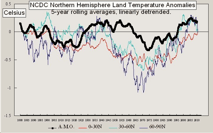
Well, the 'limpy' bit that bottoms out in 1970 drops far earlier than Amo but that isn't a problem because it isn't what were looking for - th1970 dip is the kid with the limp (that is unless Amo was on holiday for some reason in 1910). So it's the earlier bit that bottoms out in 1910 is where we should be looking.
60-90N - That doesn't really drop into the 1910 dip. It's sort of already there.
30-60N - That doesn't really drop into the 1910 dip at all but stays up until 1940.
0-30N - That does dip down to 1910 but sort of stays down from there all the way to 1970. If we decide the levelling off 1910-40 is the bobble on Amo's hat, then we'd be adding a contirbution to the peak-to-peak Global Amo wobble of 0.1C x 9% of global area = potentially 0.009C max. But can we identify it as Amo just from the bobble on his hat? -
MA Rodger at 18:14 PM on 16 June 2013The anthropogenic global warming rate: Is it steady for the last 100 years? Part 2.
With the HadCRUT4 profile evident interannually on the T&ZH13 MLR results in Fig 5b, it eventually dawned on me that it was odd the same profile wasn't evident in fig 5a. So I did a quick scale of that graph and for comparison also the HadCRUT3 results from Foster & Rahmstorf 2011.
So why does the introduction of AMO into the MLR re-introduce HadCRUT4 wobbles? Is it the Sol, Vol & ENSO signals in AMO cancelling out their input into the analysis?
-
Sceptical Wombat at 17:31 PM on 16 June 2013Peak Water, Peak Oil…Now, Peak Soil?
Putting more carbon into soil will improve the quality of the soil and should be done for that reason. However as a method of reducing CO2 in the atmosphere it makes little economic sense.
To keep organic carbon in the soil each extra ton of carbon must be accompanied by 80 Kg of nitrogen, 20 Kg of phosporous and 14 kg of sulphur which in Australia would have a total cost of about $250. Stubble generally contains small amounts of these nutrients ( with the exception of legume stubble which is relatively rich in Nitrogen) so they would have to be added in some other way.
-
Peeve at 17:11 PM on 16 June 2013Heartland's Chinese Academy of Sciences Fantasy
You can tell Cook's work hurt the denialists movement as they have responded rapidly to muddy the waters. Their 'science is not settled' meme is shattered and they must work hard to salvage something.
Personally I have used the retort to denialists 'so you know better than 97% scientists do you?' to be very effective. There is no need to be logical as they are impervious to reason, but a sharp put down works wonders.
-
panzerboy at 16:22 PM on 16 June 2013Peak Water, Peak Oil…Now, Peak Soil?
'“It takes half a millennia to build two centimetres of living soil and only seconds to destroy it,” Glover said.'
In Iceland, I believe that statement, in Brazil or Indonesia?
I have no idea, perhaps this rate of soil growth of 0.04mm/yr IS constant everywhere on the planet but my spidey-sense says no. Anyone know for sure?
-
grindupBaker at 11:30 AM on 16 June 2013Heartland's Chinese Academy of Sciences Fantasy
"...man is responsible for catastrophically warming..." S.B. "...man might become responsible...". Guy quoted seems to be a useless pessimist.
-
Ken in Oz at 11:19 AM on 16 June 20132013 SkS Weekly News Roundup #24A
If the US is anything like Australia then a big contributing factor to unwillingness of governments to commit to nuclear as emissions solution has to be entrenched climate science denial and obstructionism within conservative politics; plenty of criticising environmentalists for failing to push for nuclear from there, (pleasing to pro-nukers), but an absence of actual commitment to nuclear to replace fossils fuels (should be dispeasing but pro-nukers are given to clutching at straws).
This ought to be clear evidence that they are fair weather friends at best, and, given an absolute (in Australia) commitment to protection of fossil fuels embodied in their climate policy obstructionism, actually enemies of nuclear to replace them. So we get the argument - "If emission are a problem then they (environmentalists) should push for nuclear" being combined with (never actually stated out loud) "emissions are not a problem so we are not going to push for nuclear". Sorry but climate/energy is not about what greenies should do but about what mainstream politicians should do.
If you think nuclear is the best climate solution then you will gain more and sooner by making it clear to your conservative reps that climate science denial is absolutely unacceptable. I believe it will be more effective than fighting against anti-nuclear greenies because nuclear's biggest obstacle is weakness of support, not strength of opposition. Those conservatives are still closer to the centre of mainstream politics than green extremists and have far more clout.
Once their obstructionism isn't tenable anymore they are more likely to actually support nuclear. As long as their aim is to protect fossil fuels they never will.
-
william5331 at 10:57 AM on 16 June 2013Heartland's Chinese Academy of Sciences Fantasy
Have you seen Bill Maher's take on think tanks. Too funny.
http://www.youtube.com/watch?v=VcJohfS4vTQ
-
Synapsid at 09:24 AM on 16 June 20132013 SkS Weekly News Roundup #24A
ClimateChangeExtremist,
Again, thorium reactors do indeed produce weapons-grade material; we hear far too often that they don't.
Thorium will not support a chain reaction. Bombarding thorium 232 with neutrons produces uranium 233, which will, and that is what happens in a thorium reactor. Attempts to build a U233 bomb in the 1950s saw low yield because of radiation from U232, another result of the neutron bombardment, and its decay products, which triggered premature fission. U232 is difficult to separate from U233 but it is easy to separate from the parent of U233 (protactinium 233). The Pr233, isolated, decays into U233 with no impurities, which can indeed run a reactor but which also can be used to build a bomb. A research reactor can be used for the neutron bombardment of thorium.
The 12 December issue of Nature has an article by four British nuclear engineers which outlines two standard protocols for separating the protactinium from U232.
Thorium reactors would be a proliferation hazard just as uranium reactors can be.
-
kiwipoet at 07:52 AM on 16 June 2013Peak Water, Peak Oil…Now, Peak Soil?
A timely story. Note story with similiar focus and discussion on Hot Topic. Good video too.
http://hot-topic.co.nz/the-answer-lies-in-the-soil-you-have-to-have-a-sense-of-humus/
-
JohnMashey at 07:43 AM on 16 June 2013Heartland's Chinese Academy of Sciences Fantasy
Remmber: Heartland is a 501(c)(3) tax-exempt public charity, and its funders wer able to reduce their taxes via their gifts. Hence, American taxpayers in effect subsized this China fiasco. For some history, including some of the funding follies, see Fakery 2.
-
Nick Palmer at 04:20 AM on 16 June 2013Heartland's Chinese Academy of Sciences Fantasy
I find it quite funny that the arrogant types at Heartland have upset the Chinese so much. Diplomatic incident anyone? They've got so used to slagging off climate science, they just got too cocksure and went too far
-
ShaneGreenup at 02:44 AM on 16 June 2013Heartland's Chinese Academy of Sciences Fantasy
Either they can't remove the Press Release, or they simply forgot to take it down when they took the PR off their own website:
http://rbutr.com/rbutr/WebsiteServlet?requestType=showLink&linkId=96631
(Link to rbutr so avoid linking to the PRWeb page itself) -
JARWillis at 02:44 AM on 16 June 2013Heartland's Chinese Academy of Sciences Fantasy
What are the deniers actually saying?
If 80% of people tell you you are driving towards a precipice, sane people at least slow down. At 97% most would probably stop. When the deniers knit themselves up in arguments about percentages here, and what kinds of scientific papers you include in your analysis, at what level are they actually happy for us all to hurtle onwards, carrying their children with us?
-
dana1981 at 01:21 AM on 16 June 2013Heartland's Chinese Academy of Sciences Fantasy
Dumb Scientist - thanks, I've updated the Heartland links to the WebCited version. Heartland is now backtracking fast:
"To be clear, the release of this new publication does not imply CAS and any of its affiliates involved with its production 'endorse' the skeptical views contained in the report."
Damage control mode!
-
r.pauli at 01:10 AM on 16 June 2013Heartland's Chinese Academy of Sciences Fantasy
Denialist propaganda is a dangerous weapon - when weilded by psychopaths it destroys the future -- an unintentional mis-fire at the misinformed - mostly children.
It is a loose cannon firing wildly in every direction.
-
citizenschallenge at 00:43 AM on 16 June 2013Heartland's Chinese Academy of Sciences Fantasy
Nice informative post Dana, thanks for getting this out there.
FWIW since it makes a good bookend for this saga I've reposted it at.
"Heartland Institute caught in a lie - Chinese Academy of Science objects"
http://whatsupwiththatwatts.blogspot.com/2013/06/heartland-institute-caught-in-lie.html
-
timallard at 23:48 PM on 15 June 2013The last time carbon dioxide concentrations were around 400ppm: a snapshot from Arctic Siberia
"The fact that there exists strong evidence for past major warming and its consequences in both polar regions suggests an interconnectivity between the poles, with the implication that these are effects occurring on a global scale."
Consider that right now the planet increases heat retention daily, radiative forcing, and that the flucuations in CO2 are not affecting this much at all due to it still being a rising value. Because of this the atmosphere is now moving heat north and cold south, and the reverse in the southern hemisphere faster and more directly due-north, due-south over both poles as a result.
Both poles are doing this and indications of this are the late season snow in both Europe and the Midwest at this time. These are not mysterious but a by-product of the atmosphere being a heat-transfer system vainly trying to maintain thermal balance until we remove the cause.
This process is to me what keeps global temperatures from rising at this time, it's like we're using an old-style ice-box to cool the house and once the ice is gone nothing is left to cool the planet, ice melted and permafrost thawed.
Therefore global temperature is not a good short-term indicator, it's not predicitive of what's going on, an example, 30-years ago near Disco Island only dogsleds could be used for 6-months of the year, today hunters use their fishing boats to hunt seal, very few use their sleds anymore. What model predicted this?
Further, observing jetstream paths for many years I noticed that many times the air arriving in the Disco Bay area came from the Tropic of Cancer latitudes in the Pacific, gained latitude as moved east and continued NNE to pass over Disco Bay. This versus the cold-period regime that brought very cold air from the north for especially the three coldest months Jan-Mar. From locals they have observed this from being on average -30C historically to today where it's rare to have below -10C, a +68F/20C rise in average temperature.
This easily explains the loss of sea-ice in this area and it's from new jetstream paths being taken quite often in winter which was not predicted by models, thus my reason for bringing it up. That is to recognize that the atmosphere is doing many north-south pieces of jetstream moving the cold to the equator and heat to the poles, this needs to be included in models, we have a new circulation pattern now, the atmosphere is being driven by the radiative forcing regardless of what global temperature registers as it's being held back until the cold storage from the previous ice-age is gone.
So, I'd suggest to modelers & others, that heat-transfer is the main driver now and without assessing the volume heat transfer by analyzing air masses, their volume, temperature, humidity and direction there's no way to be predictive of these on-the-ground radical changes such as at Disco Bay.
Prev 904 905 906 907 908 909 910 911 912 913 914 915 916 917 918 919 Next


