Recent Comments

Prev  942  943  944  945  946  947  948  949  950  951  952  953  954  955  956  957  Next

Comments 47451 to 47500:

47451. Tom Curtis at 01:40 AM on 15 March 2013
       Drost, Karoly, and Braganza Find Human Fingerprints in Global Warming
       

       Observed trends, Jan, 1961- Dec, 2010:

       GISS: 0.151 +/- 0.027 C/decade.  (Upper confidence interval: 0.178 C/decade)

       NOAA: 0.142 +/- 0.025 C/decade.  (Upper confidence interval: 0.167 C/decade)

       HadCRUT3:  0.140 +/- 0.029 C/decade.  (Upper confidence interval: 0.169 C/decade)

       HadCRUT4: 0.139 +/- 0.027 C/decade.  (Upper confidence interval: 0.166 C/decade)

       So, one out of four temperature indices just fails to scrape in the confidence interval.  That index is known to not have global coverage, and in particular to have poor coverage of the Arctic, Asia, and North Africa (all areas showing very high temperatures in 2010)  Indeed, the only index of the four to have truly global coverage is also the one that most closely matches the predicted trend.

       Kevin does point toward a genuine problem, however, though it is not what he thinks it is.  It is about time climate scientists started using a HadCRUT3 (or 4) mask on their predictions when comparing predicted temperatures and trends to the Hadley products.  It is known that they do not have global coverage, and it is known that that effects the temperature trends.  The continued reliance on HadleyCRU products without produceing a Hadley mask prediction is the equivalent of comparing North American continent temperature predictions to USHCN CONUS temperature products.  It is not a prediction of the thing being measured.

47452. Kevin8233 at 00:35 AM on 15 March 2013
       Drost, Karoly, and Braganza Find Human Fingerprints in Global Warming
       

       Due to those overpredictions, on average the models simulate a 0.167°C per decade average global surface warming trend from 1961-2010, whereas the observed trend is approximately 0.138 ± 0.028°C per decade, approximately 20% lower.

        

       The max of the observed trend is 0.138 + 0.028 = 0.166.

       What does it mean when the max of the observed trend is less than the model's prediction?

       Since this covers 49 - 50 years, it is a substantial amount of time.  I would say that the model is out of whack!

        

47453. Hans Petter Jacobsen at 21:04 PM on 14 March 2013
       Living in Denial in Norway
       

       I agree with Esop @19 that the return of cold winter weather has affected the opinion in Norway. Cross country skiing, which requires cold winter weather, is still a part of the national identity for many Norwegians, myself included.

       Norway is a young nation, and polar explorers like Fridtjof Nansen and Roald Amundsen were important for the national identity both before and after Norway was separated from Sweden in 1905. Nansen tried to reach the North Pole in an expedition that lasted for 3 years. They did not manage to ski all the way to the Pole, but he and his men survived, and they were heroes when they returned home. Most Norwegians know about the expedition and the hardships that the men went through in the Arctic ice. An ice free North Pole may therefore change people's opinion. In 2010 a modern Norwegian explorer sailed around the Arctic in a small fiberglass sailboat, and he got much attention in the media. It took Amundsen 3 years to sail the western part of this route and 2 years to sail the eastern part of it, despite his vessels were designed for the pack ice. I assume that someone will sail to the North Pole in a small fiberglass sailboat soon, and that this will have a greater impact on the opinion in Norway than anywhere else.

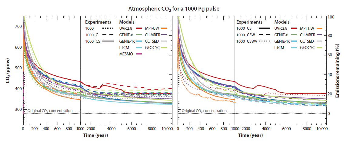
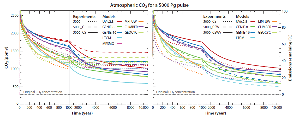
47454. MA Rodger at 19:27 PM on 14 March 2013
       No alternative to atmospheric CO2 draw-down
       

       Hi Tom Curtiss @49.

       Thanks for turning Archer's figure 1 round the right way up. In the past I have always met it on its side which does make fully appreciating its content a bit stressful.

       The text of Archer 2009 is a different matter, although you did get me checking who was right.

       The pulses of CO2 he models are in Pg carbon (GtC in my-speak) and not in Pg CO2. Archer describes the size of the smaller of these pulses thus "For comparison, humankind has already released 300 Pg C and will surpass 1000 Pg C total release under business-as-usual projections before the end of the century." Archer's 300 GtC for human releases is surely low, even for 2009 (which if you tot them up would have been 350 GtC back then according to CDIAC, and now over 400 GtC). It also ignores land-use emissions which tot up to a further 160 GtC according to CDIAC which makes today's total release probably over 560 GtC.

       Thus under BAU, I would put the 1,000 PgC emissions milestone as arriving, not as Archer says "before the end of the century", but by mid-century.

       The larger 5,000 PgC pulse he equates to burning of all FF reserves including coal (although likely tar sands & fracked gas probably don't feature). Fuel reserves are always a nightmare, with the numbers quoted ranging from 'reserves from current holes in the ground using current extraction methods' all the way to 'estimated potential global reserves extractable using theoretical methods.' I do think Archer is at the high end of these different figures when he says the 'entire reserviour of fossil fuel' equates to his 5,000 GtC. A figure of 760 GtC (2,795 GtCO2) is encountered commonly which I interpret as 'known reserves less tar sands & fracking'. There is as well resulting carbon feedbacks from permafrost so BAU for 60 years would easily see resultant total accumulative carbon emissions up to 1,500 GtC.

47455. Leto at 16:43 PM on 14 March 2013
       Water vapor is the most powerful greenhouse gas
       

       gws #154, thanks.

47456. KR at 13:30 PM on 14 March 2013
       Water vapor is the most powerful greenhouse gas
       

       Tom Curtis, Jose_X - If I am referring to running the same experiment in steps (one or many), and you are referring to something else entirely (with/without feedback, under different conditions, for example), then my apologies, that's apples and oranges. Different questions entirely, and comparing the two is not particularly relevant. 

       What I was discussing is that a numeric analysis of 400ppm will be the same as another analysis of 400ppm, all other things held constant (including the presence/absence of feedbacks and whether or not sufficient time for equilibrium is allowed), regardless of other calculations, and that interim values for GHG levels will and must fall somewhere between the 0ppm and 400ppm numbers. Not retaining feedback levels for one forcing level over to another, which is invalid, but running each step of the experiment under the same conditions as the final 400ppm evaluation. To be really clear, I'm speaking of total forcings, not deltas, as the deltas will be dependent on the temperature at the time of the delta - if you are looking at varying temporal evolution without equilibrium, all bets are off. 

       But I'll freely admit that I may not be fully following the conversation - I'm still quite unclear on what Jose_X wishes to investigate, what issues he's seeking insight into. 

47457. Tom Curtis at 11:12 AM on 14 March 2013
       Water vapor is the most powerful greenhouse gas
       

       KR @156, I think you aren't sufficiently considering the fact that the radiative forcing between two concentrations is the difference in TOA radiative flux at equilibrium for one concentration and the TOA radiative flux for the other concentration with all other values (ignoring the stratosphere) retaining the equilibrium values for the other concentration.

       In fact, one relevant experiment for assessing a related issue has been done.  In Schmidt et al, 2010 they compared the effect of adding a slug of IR active compounds (and clouds) to a pristine atmosphere (N2 and O2 only), and the effect of removing the same size slug from an atmosphere with the composition found in the 1980s.  Because CO2 has virtually no overlap with any factor other than water vapour and clouds, that experiment effectively determines the RF of adding 340 ppmv to an atmosphere with no CO2; and the RF of removing 340 ppmv from an atmosphere with 340 ppmv of CO2.  The result for adding the CO2, ie RF(0→340), is 38 W/m^2.  The result for removing the CO2, ie, RF(340→0), is 22 W/m^2.  The difference is because, in the very cold climate with 0 ppmv CO2 after equilibriation, there is virtually no water vapour and no clouds in the atmosphere (not quite true but close enough for exposition).  In the case of addition, that means there is no overlap, and the full effect of the addition can be experienced.  In the case of removal, the full load of water vapour and clouds are retained in the atmosphere because this is a no feedback situation.  So, not only does the RF of a large slug not equal the RF of the sum of a series of small slugs of the same size, but the RF varies depending on whether you are adding, or removing the slug.

       This does not mean that the equilibrium temperature will differ for a given concentration of CO2 depending on whether you arrive at that concentration by increasing or decreasing CO2.  To the extent that the difference in RF between the two methods is a consequence of the overlap with water vapour and clouds, as the vapour pressure of water in the atmosphere adjusts to a reduced (or increased) temperature, the extent of overlap will equalize.  So, λ also differs between the two cases such that λ'RF(0→340) = λ"RF(340→0).

       Again, this later property is not necessarilly true, and is not true for some values of CO2 concentration and for Earth System Climate Sensitivity, with a bifurcation between snowball earth and non-snowball earth states resulting in λ'RF(a→b) ≠ λ"RF(b→a) for some CO2 concentrations, a and b.

       Finally, and as you point out, the simplified formular does apply within error, and has been shown to apply for a large range of CO2 concentrations close to the present value (ie, from about 150 ppmv to several thousand ppmv at least), and in that range, to a close approximation, it does not matter whether you increase or decrease, or change the concentration in a single slug or by increments, the answer will be the same.

47458. Eric Grimsrud at 11:05 AM on 14 March 2013
       State Department Downplays the Climate Impact of Keystone XL
       

       To John Hartz and John Cook, 

       I would be pleased as well as honored to serve as a volunteer on the SkS author team.  I consider SkS and Climate Progress to be the best I have noted to date for updates on climate change issues, both scientific and political.  W.R.T. my own personal efforts, see ericgrimsrud.com and ericgrimsrud.wordpress.com.   

47459. dana1981 at 10:05 AM on 14 March 2013
       State Department Downplays the Climate Impact of Keystone XL
       

       john @4 - yes thanks, that should have said 'barrels', not 'gallons'.  Correction made.

47460. shoyemore at 08:52 AM on 14 March 2013
       State Department Downplays the Climate Impact of Keystone XL
       

       Given Obama's poor track record, I feel Keystone will be approved later in the summer. Also, knowing Obama, there will be big compensatory gestures to the "green" movement, maybe to do with carbon emissions or coal exports.

       I am not sure if that will be enough. We will need to see the final package.

47461. Tom Curtis at 08:46 AM on 14 March 2013
       Water vapor is the most powerful greenhouse gas
       

       Jose_X @155:  In taking multiple steps in the first experiment, the atmosphere was never allowed to equilibriate.  As a result, the mean global surface temperature, water vapour content of the atmosphere, etc, was constant at 0 ppmv CO2 levels throughout the experiment.  You could, it you want run multiple experiments, where in each experiment you allow the atmosphere to equilibriate at 0 ppmv CO2, then add slugs of 40 ppmv CO2, 80 ppmv CO2, 120 ppmv CO2, etc, but you would get the same result.  That result is the RF(0->40), RF(0->80), etc, which allows you to see the incremental difference in RF not just for the step from 0 to 400, but for all the intermediate steps as well.

       In fact, thinking about it, it would be best to run 10 experiments.  One in which you set CO2 to 0 ppmv, and allow it to equilibriate, then incrementally increase to 400 ppmv without allowing equilibriation between each step.  One in which you set CO2 to 40 ppmv, then incrimentally increase without allowing equilibriation, and so on.  This series of experiments would allow you to calculate the RF(0-40), (0-80), ... . ((0-400); (40-80), (40-120), ..., (40-400), ... ,(360-400).  

       Doing so, I suspect you would find the difference between RF(120-400) and the sum of the differences RF(120-160), RF(160-200), etc would be small.  That is, most of the H2O/clouds/CO2 overlap would arise in the first few increments because the first few increments of CO2 have the largest effect on temperature and hence on CO2 content.  If, however, we pushed the experiments out to 2000 ppmv, the difference introduced by each incremental step would start rising again as the increase in vapour pressure of water with increase in temperture rises rapidly above 40 C (ie, typical tropical tempertures with very high CO2).

       Finally, your suggested experiment is no different than mine, except that it does not obtain intermediate values for the RF relative to 0 ppmv.     Consequently, by my analysis, it would also show the RF(0-400) to be greater than the sum of the incremental radiative forcings.

47462. Jose_X at 08:29 AM on 14 March 2013
       Water vapor is the most powerful greenhouse gas
       

       KR 156 >> How could the forcing at 400ppm possibly not equal the forcing at 400ppm?
       
       I'll quote Tom Curtis 152:
       > b) Radiative Forcing is not a concept in a basic physical theory, but rather a concept used in calculating the approximate consequences of the complex interactions of basic physical theories.  Consequently what is required of it is that it be sufficiently useful in its range of operations - which of course, it is.
       
       One might ask in Calculus, how could the derivative of x^3 + x^2 not possibly be the same as the derivative of x^3 plus the derivative of x^2? Well, the derivative operator was designed, among other things, to be linear. But we can design many algorithms/operators that don't have that feature. In fact, it's not really clear that an algorithm has such a property until it is "proven" in a rigorous analytical sense.
       
       The odd thing to me about RF is that it disappers after equilibrium is reached. By looking at equilibrium radiation at TOA or on the surface, you can't tell. In fact, there are many independent variables that go into deriving RF and if any of those are left out of the analysis, you really can't recapture that value. And improvements in our understanding in the future might even lead to different algorithms that would derive different RF. Each time we engage in a new algorithm, arguably, we should try to prove that certain mathematical properties exist. I don't think it is obvious that a complex algorithm dependent on numerous factors would automatically be well-behaved in any particular sense of the word.
       
       OK, let's assume we are going from a given starting concentration of CO2 to another where the RF value "at" each path point can be modeled by roughly the same logarithmic function (dependent on a reference point). We can take multiple paths there.
       
       Question: is it obviously true that a*ln(b*(x_1/x_0)) + a*ln(b*(x_2/x_1)) = a*ln(b*(x_2/x_0)) for all x_1 and x_2? At best we should perform the algebra first to be sure (or to show instead that the path does matter). Here I believe the path doesn't matter.
       
       What if the approximating functions used along the partitioning path were entirely different from each other?
       
       Also, we can even look at forcings by different gases and ask, what if the gases are added in different orders and quantities?
       
       If the approximation method used to address any of these questions gives a result that the partition chosen does matters, one can't argue that if we simply had used the true and best method (codes) then it all would have worked out because it would adhere to reality, etc, etc. Every algorithm/calculation is an approximation of reality to some degree. Why should today's current best procedure necessarily be the best we will ever get so to allow that logic to work?
       
       OK, since I am writing before carefully reviewing the logic of this comment sufficiently, I too would certainly appreciate comments, complaints, etc. I heretoforth reserve the right to backtrack through an unlimited number of "undos".
       
       PS: "KR" and "RF" can get a little confusing. They each have an R and that looks like the other letter, a verticle line with two smaller lines connected each in at least a quasi horizontal position.

       KR, thanks for the modtran link. I'll see if I can make use of it.

47463. john mfrilett at 07:36 AM on 14 March 2013
       State Department Downplays the Climate Impact of Keystone XL
       

       I think this may be in error by a factor of 100, "Using 600-gallon tank cars".  Tank cars can have capacities of up to 60,000 U.S. gallons of fluid. 

       Moderator Response: [AS] I believe that is an error, it should say "barrels" instead of "gallons". The SEIS uses 600 barrels per tank car, about 19,000 US gallons.
47464. Hans Petter Jacobsen at 07:10 AM on 14 March 2013
       Does Norway lack political commitment to renewables?
       

       StBarnabas comment #1 inspired me to look more into the possibilities for power exchange between Norway and Europe.

       A report from a seminar arranged by CEDREN gives a good overview of how Norway, Germany and the UK may balance power using the hydro reservoirs in Norway. The report states that "Demand for Norwegian pumped-storage hydropower is rising." The UK has signalled a long-term demand for balancing power in the range of 15–20 GW. Germany has indicated a substantially greater need (20-60 GW). The Norwegian Statnet states that a balancing power regime of up to 20–25 GW is obtainable from a Norwegian technical standpoint. There are more details in the report.

       A report form Zero states that "With hydro reservoirs of 84 TWh, Norway holds about 50 percent of  Europe’s hydro power storage capacity." The report focuses on balancing power between Germany and Norway. Today Germany has 30 hydro power pump storage stations with a total capacity of 6.8 GW. When the magazines are fully loaded, they can run for 4-8 hours and produce a total of 0.04 TWh. A totally 100% renewable electricity system in Germany in 2050 will require 76 TWh of reimport each year, which corresponds to almost the total storage potential of the Norwegian hydro power magazines. A maximum capacity of 50 GW in- and output is required. To obtain the approximately 50 GW input and output capacity, the turbine capacity of Norwegian power plants would have to be expanded, apart from stepping up pumping capacity. Current installed hydropower capacity in Norway is 28 GW (The numbers in the report vary a little). Statkraft carefully indicates a potential from everything between 30 to 85 GW, but an interim report states that Norway could supply up to 20 GW of balancing hydropower. 

       The Zero report states that "The construction of new hydro reservoirs in new areas in Norway for electricity export is highly unlikely. The most discussed solutions in recent reports on balancing options are pump storage and expansion of existing hydro power plants". The report also discusses the opposition among people in Norway against new power lines due to visibility in the landscape.

       I have played with some numbers to set 20 GW balancing power in perspective. The 500 million people in the EU countries consume approximately 2600 TWh each year, which is approximately 300 GW on average. The energy capacity in the Norwegian hydro reservoirs is 84 TWh, which corresponds to 20 GW power for 4200 hours, i.e. for almost half a year.

47465. Tom Dayton at 07:00 AM on 14 March 2013
       State Department Downplays the Climate Impact of Keystone XL
       

       There's a really good article on Keystone by Ed Dolan in, of all places, OilPrice.com.  The key quote:

       It is very likely true that blocking Keystone would not stop the development of Canadian oil sands in its tracks. Whether or not it proceeds at “about the same pace” is another question. If Keystone is, as its backers argue, the lowest-cost way to get Canadian bitumen to market, then failing to approve it would raise the delivered cost of the product. Other things being equal, we would expect that to slow development. On the other hand, if Keystone is not the least cost means of delivery, or if its cost advantage is trivial, then it would seem that we would gain little by building it. You can’t have it both ways.

       I highly recommend reading the whole article, which recommends full-cost accounting for greenhouse gas emissions (i.e., carbon tax).

47466. KR at 05:45 AM on 14 March 2013
       Water vapor is the most powerful greenhouse gas
       

       Jose_X - "Question: Does the sum of all 10 RF measurements made at step 2 in Experiment 2 equal the single RF measured from Experiment 1?"

       Yes, rather by definition. The radiative forcing of 400ppm CO2 will be the same no matter the path; the increments at whatever slicing have to add up to the same number. 

       How could the forcing at 400ppm possibly not equal the forcing at 400ppm? With forcings at different intermediate concentrations (as the first one or two of your small steps may still be in the linear range, not logarithmic, depending on step size) falling somewhere between the 0ppm and the 400ppm levels??? I cannot conceive of the math working out any other way...

       If you want to play around with these numbers, you might try out one of the online MODTRAN packages. Keep in mind that the 3.7 W/m² forcing change per doubling of CO2 (curve fit in the log range) was calculated from multiple numeric runs at different latitudes (Myhre 1998). 

       In regards to the CO2/water overlap, again, there is no substitute for actually doing the math. Which in this case means line-by-line numeric codes using a multiple layer model; I believe MODTRAN-style calculations converge for any particular conditions at about 20 layers or so, with additional segmentation not greatly affecting the numbers. There is no simple analytic formulation - the radiative effects depend on GHG concentration (water vapor falling off faster than CO2), altitude, and temperature at each level, and as in ordinary differential equations, a numeric approach (similar in concept to Runge-Katta) is the most appropriate. 

47467. John Hartz at 05:04 AM on 14 March 2013
       State Department Downplays the Climate Impact of Keystone XL
       

       Eric Grimsrud:

       Thank you for sharing your thoughts and for the links to your most recent op-ed. If you are interested in joing the all-volunteer SkS author team, please let John Cook know. Your background and willingness to speak out are impressive.

47468. Jose_X at 03:37 AM on 14 March 2013
       Water vapor is the most powerful greenhouse gas
       

       Tom Curtis 152:
       Concerning item 2:
       
       The two experiments might answer part of what I was asking, but I am interested in at least one variation in order to try to factor out the water/CO2 overlap so to answer the main question I had.
       
       First, I am not sure why to get RF(0->400) in experiment 1 (where you didn't run feedbacks), you went through a sequence in steps of 40? The key to the main question I had might be there. Since the question of CO2 contribution was a vehicle to address the partion equivalence question (ah, the truth comes out), I think I would now like to "run" a new pair of experiments, each of which avoids running feedbacks.
       
       Experiment 1:
       1- allow the GCM to reach equilibrium with 0 CO2
       2- step to 400 CO2 and measure the RF.
       Experiment 2:
       1- same as step 1 for Experiment 1
       2- step to 40 CO2 and measure RF
       3- allow equilibrium to be reached
       4- repeat steps 2 and 3 but increasing the CO2 concentration each round by 40.
       5- the repetition ends when at step 2 we have stepped to 400 CO2 and measured RF.
       
       Question: Does the sum of all 10 RF measurements made at step 2 in Experiment 2 equal the single RF measured from Experiment 1?
       
       Later I intend to look at 2 more experiments where each run feedbacks, but I'm not ready to present that example and associated questions. I will be interested in the imbalances at TOA as the feedbacks are in effect (transients towards equilibrium). One question now: Is it meaningful to ask for the RF value of say H2O (a feedback of CO2)?

47469. Philippe Chantreau at 02:09 AM on 14 March 2013
       The educational opportunities in addressing misinformation in the classroom
       

       Thanks for doing the leg work Tom. My figures closely match your results, not surprisingly as they came from reliable sources. As always when physical reality is considered, there is a right answer and it's not all a matter of opinion. Because combustion is not perfect and there is more than just C and H in Jet fuel, the actual ratios are about 70% CO2, a little less than 30 % water and less than 1% SO, NO, CO and others. The links above have details. Elektroken was way off.

47470. Eric Grimsrud at 01:58 AM on 14 March 2013
       State Department Downplays the Climate Impact of Keystone XL
       

       Living in the fuel rich state of Montana, it is difficult to convince our elected officials to turn down our spigots for the export of gas, oil and coal.  As a former atmospheric scientists, I nevertheless do my best to make the argument - based on the science involved.  FYI,  my latest attempt can be seen at http://missoulian.com/news/opinion/columnists/global-warming-is-our-greatest-immediate-challenge/article_199255c2-6638-11e2-b352-0019bb2963f4.html. My short piece follows several recent presentations by Kevin Anderson of Great Britain (such as the one at http://www.climatecodered.org/2011/12/professor-kevin-anderson-climate-change.html) which make brutally clear the urgency of the issue. 

47471. gws at 22:08 PM on 13 March 2013
       Water vapor is the most powerful greenhouse gas
       

       Leto, good question.

       Essentially, you answered the question yourself already, through your example.

       The atmosphere is a fluid, much like the water behind the dam. So it behaves like the dammed water, aka mathematically there is no difference here. Scale, however, is important.

       Your example illustrates two aspects:

       1. Residence time: The dam is in equilibrium, discharging as much water as it takes in. Residence times are e-folding times (time to 1/e) and represent the solution to their defining equation, namely tau =  abundance / removal rate. That is long in the dam case, but relatively short in the atmosphere case. In the latter case, tau varies strongly by location, for example latitude (high cloud density and rain (=removal) rates in the tropics!)

       2. Local vs. global viewpoint: You cannot instantaneously mix a local emission into a larger volume. As everyone knows from looking at car exhaust ("instant" injection), high water vapor amounts condense very quickly  when the surrounding air cannot support that much water vapor, such as during cold winter days. Only if your heavy water mixed uniformly and instantaneously into the large dammed water volume (which it does not) would its residence time be equal the dammed water residence time.

       Increasing atmospheric temperature is equivalent to slowly raising the dam wall height in your example, allowing the lake behind it to hold more water over time. Aka, during that time, the dammed water (the atmophere) is not in equilibrium.

       Locally/regionally, a stronger greenhouse effect does indeed occur where atmospheric water vapor is in higher concentration (air-temp. during humid nights drops slower than during dryer nights; think of how cold a desert can get at night). One needs to integrate over these effects to get the global picture. There is not one scale (tau) fits all, there are many scales that matter.

47472. Leto at 21:02 PM on 13 March 2013
       Water vapor is the most powerful greenhouse gas
       

       Some interesting discussions in this thread, thanks. Could someone please clarify one small issue for me? Early in this multi-year thread, mention was made of the short residence time of water vapour in the atmosphere. It was also suggested that, given a specific and stable temperature-pressure combination, the atmosphere responded "almost instantly" to the addition or subtraction of water.
       
       Tom Dayton (#69) wrote...What does primarily limit the amount of water vapor in the (Earth's) atmosphere is the atmosphere's temperature. At a given temperature, adding more water vapor "nearly instantly" forces water vapor to drop out of the atmosphere. "Nearly instantly" in this context means "so fast that there is no time for significant atmospheric heating from the extra water vapor."
       [...]
       What's needed to increase water vapor for more than 10 days is an increase in atmospheric temperature.
       
       I would like to understand how quickly the atmosphere responds to a sudden influx of water vapour - say, from an anthropogenic source - does it really depend on the mean residence time of water vapour, and is 10 days a reasonable approximation of water vapour MRT? (It's probably not important in terms of AGW theory - 10 days is as good as instant anyway - but I am curious anyway.) My understanding of mean residence time (MRT) is the mean time that each water molecule stays in the atmosphere. (Speaking in terms of half-lives would seem more natural to me). Intuitively, I would have thought the atmosphere responded faster than the residence time suggests - couldn't the added water displace other water to reach equilibrium again even faster than the MRT? But my intuitions might be way off, so I'd be happy to be educated by those who have studied this.
       
       To pick a simplistic example (just to illustrate what I am asking, not because it is anything like the climate): take a dam that is always full, right up to the overflow wall, because of an inflowing stream. If I add a bucket of heavy (deuterium-rich) water, it might mix into the much larger volume of the dam such that the added molecules have a long MRT, measured in months. There would be an earlier distributive/mixing phase, from diffusion and convection, followed by an exponential decline dependent on the outflow from the dam. But the dam could discharge the extra volume (not the actual heavy water molecules from the bucket) very quickly, perhaps in minutes.
       
       So, is the atmosphere's return to its pressure-temperature-determined water content rapid, like the dam losing the added volume of water, or is it more like the dam eventually losing the radio-labelled molecules themselves? And does the answer change for different parts of the atmosphere?

       Thanks in advance.

47473. gws at 19:48 PM on 13 March 2013
       Does Norway lack political commitment to renewables?
       

       OPatrick

       I think it is important to make a clear difference between demand and supply. That demand will increase is clear when you look at your typical developing country. During the developing phase and decades beyond there is a clear correlation between growth and energy use (the decoupling occurred late in the western world). China and India are prime recent examples. As long as such development is fed by fossil fuels, as it largely is at this point in time, the fossil fuel industry promotes such growth.

       The sentence in question is therefore one I have heard mostly from industry representatives. It seems a bit odd to see it in this article, but keep in mind that the defining adjective here is "global". Then, the answer to your question is likely "yes".

       What we should not accept though is that the demand is supposed to satisfied by fossil fuels. Much (all?) of the demand can instead be satisfied by renewables and efficiency as has been pointed out in many monographs. But that takes political and societal will, as it entails a major shift away from the current fossil fuel infrastructure we are so content with ...

47474. OPatrick at 18:54 PM on 13 March 2013
       Does Norway lack political commitment to renewables?
       

       Since we know that the global demand for energy will increase dramatically over the next 30 years

       Is that certain beyond doubt? Should we be accepting it as certain beyond doubt?

47475. Tom Curtis at 18:50 PM on 13 March 2013
       Water vapor is the most powerful greenhouse gas
       

       Jose_X:

       1)  The total forcing of current CO2 concentrations relative to zero concentrations is, by best estimate, 38 W/m^2.  This is different from the all sky contribution of CO2 to the total greenhouse effect because of the overlap with the contribution from H2O and clouds.  This is different from the all sky contribution of CO2 to the total greenhouse effect because of the overlap with the contribution from H2O and clouds.  To determine the forcing, we must imagine an initial situation with, effectively, no water vapour and no clouds because of the very cold temperatures (-19 C mean global surface temperature).  Because there is minimal water vapour and clouds, there is also minimal overlap in absorption frequencies with CO2, so the forcing of adding the CO2 correlates best with single factor addition contribution from table 1.

       Clearly calculating this value relies on using a Global Circulation Model (GCM), and the use of different GCM's will give slightly different results.  Because we are reliant on GCMs, this represents our best theoretical prediction, for (of course) we cannot actually conduct the experiment.

       Of interest, given the formula ΔT = λ RF (change in global mean temperature equals the climate sensitivity parameter times radiative forcing, see IPCC AR4)  The change in temperture of 33 C as a result of the greenhouse effect with a forcing of 38 W/m^2 gives λ = 0.87 C/(W/m^2), equivalent to a climate sensitivity of  3.2 C per doubling of CO2.  This is, of course, a very crude estimate, but it would be surprising of the Charney climate sensitivity was not in that ball park.  It should be noted that if we reduce the forcing (to allow for some overlaps), the estimated climate sensitivity increases.

       2)  The only way to determine the radiative forcing for a given value of CO2 for values significantly different from current values is by means of model runs on GCMs.  You would run two concurrent experiments.  In the first experiment you run the GCM with zero CO2 until it reaches equilibrium.  You then increase the CO2 concentration to 40 ppmv, holding all feedbacks constant and determine the difference in TOA flux, thus determining RF(0->40) (Radiative Forcing for a change from 0 to 40 ppmv).  You then increase the CO2 concentration to 80 ppmv and determine RF(0->80), and so on.  In the second experiment you would do the same thing, but after determining the RF for each increment, you would allow the feedbacks to vary, and run the GCM until equilibrium was obtained before introducing the next increment.  By doing this you would obtain RF(0->40), RF(40->80), etc.

       As I understand your question, you are asking whether  RF(0->40) + RF(40->80) + RF(80->120) + ... + RF(360->400) = RF(0->400).

       I think, based on the points I made in (1) above, they would not.  Specifically, RF((0->400) =~= 38 W/m^2, but because of the overlaps with water vapour, the sum of the smaller steps would be closer to the net current contribution of CO2 to the total greenhouse effect (30 W/m^2).  Specifically, it would equal the sum of the radiative forcings for each step minus the contribution to the overlap from each step but the last.  The smaller the steps you used, the closer it would approximate to the current CO2 contribution.  If you used very few steps, however, the result would not be very different from using just one step.

       What follows from this? Virtually nothing.  I would need to amend my comments above, but:

       a) The partition of current effect in cases of overlap is largely a matter of convention, and adoption of a different convention would resolve the discrepancy; and most importantly

       b) Radiative Forcing is not a concept in a basic physical theory, but rather a concept used in calculating the approximate consequences of the complex interactions of basic physical theories.  Consequently what is required of it is that it be sufficiently useful in its range of operations - which of course, it is.

       Finally, it is possible (as if this needs mentioning) that my reasoning above is faulty.  Consequently I would be very interested in any criticism of my comments.  

47476. gws at 18:38 PM on 13 March 2013
       Does Norway lack political commitment to renewables?
       

       For those of you wondering about this post, as it is seemingly not in line with what SkS "usually" posts about, here some background:

       • we want to occasionally expand from the slightly US-AUS-UK-centric focus of SkS
       • we do not necessarily endorse any opinions expressed in the article (it is a translation only)
       • two posts on Norway within 2 weeks was coincidental
       • we welcome any feedback that helps in understanding the topic better

       Thus, the first two comments here are obviously productive. Norway is a special case: while producing virtually all its own electricity from hydropower, a renewable energy source, its relatively low population alongside a large oil&gas industry make it the largest per-capita CO₂ emitter in the world (when counting fossil fuel exports in the Norwegian budget, instead of where they are burned). Norway is a major fuel supplier to the rest of Europe, recently visited again by Germany for talks about long-term energy planning. So, I guess, whatever direction Norway goes is quite relevant for the climate.

47477. Tom Curtis at 16:48 PM on 13 March 2013
       The educational opportunities in addressing misinformation in the classroom
       

       Taking dodecane (C₁₂H₂₆) as a typical hydrocarbon in kerosene, then:

       2 x C₁₂H₂₆ + 37x O₂ → 24 x CO₂ + 26 x H₂O

       Substituting in atomic masses, we get:

       2 * (12 * 12 + 26 * 1) + 37 * (16 * 2) = 24 * (12 + 2 * 16) + 26 * (2 * 1 + 16)

       or  340  + 1184 = 1056 + 468.

       So, the mas of water produced is 1.37  times the mass of fuel burned.  The mass of CO₂ produced is 3.1 times the mass of fuel burned.   And the mass of CO₂ is  69% of the total emissions by mass, with H₂O constituting 31%.

       Of course, not all kerosene is dodecane, and in most circumstances it will not combust perfectly, so these are just ball park figures, but certainly confirm Sof of Krypton and Phillippe Chantreau.

       Of course, this is just having fun around the edges.  The true rebutal of elecktron was given by KC in moderator box.  Just because elektron was unfamiliar with the literature did not give him the right to assume that scientists had not investigated the effect he just thought of in great detail.

47478. Philippe Chantreau at 14:53 PM on 13 March 2013
       The educational opportunities in addressing misinformation in the classroom
       

       Son of Krypton ,EPA lists Jet Fuel at 20.89 Lbs of CO2 per gallon. 

       http://www.epa.gov/cpd/pdf/brochure.pdf

       A gallon of jet fuel weighs about 6.8 pounds. So a pound of jet fuel produces about 3.1 Lbs of CO2. Jet engines emit about 2.3 times as much CO2 than H2O, which would put the ratio at approximately 1.3 Lb of water per Lb of jet fuel. Feel free to double check, there are multiple sources where this is examined. I don't know where Elektroken got his 5:1 figure.

         FAA figures.

       Moderator Response: [RH] Shorten link that was messing with page format.
47479. Son of Krypton at 13:58 PM on 13 March 2013
       The educational opportunities in addressing misinformation in the classroom
       

       And I see that comment didn't work at all. Well I know for next time to just use the Source section (walks away in shame)

       Moderator Response: [RH] It was an easy fix.
47480. Son of Krypton at 13:56 PM on 13 March 2013
       The educational opportunities in addressing misinformation in the classroom
       

       To put John's recommendation of refuting a myth into practice; electroken@2 wrote "Jet airplanes produce 5 pounds of water vapor per pound of fuel burned and they burn a whole lot of it"

       
       Well, it seems the science begs to differ. The FAA (2005) wrote that "Aircraft engine emissions are roughly composed of about 70 percent CO2, a little less than 30 percent H2O, and less than 1 percent each of NOx, CO, SOx, VOC, particulates, and other trace components including HAPs."

47481. Son of Krypton at 13:43 PM on 13 March 2013
       The educational opportunities in addressing misinformation in the classroom
       

       Have to say it, I exploded laughing at the Yoda link

47482. Jose_X at 11:42 AM on 13 March 2013
       Water vapor is the most powerful greenhouse gas
       

       With a good grasp of the algorithms involved to calculate a forcing, we could probably just analyze that.

       
       And if someone was actually going to carry out the computational experiment, perhaps limit the number of steps to avoid approximation error propagation from interferring.

47483. Jose_X at 11:34 AM on 13 March 2013
       Water vapor is the most powerful greenhouse gas
       

       KR, calculating the forcing for CO2 early on in the process (near 0% CO2) and continuing, eg, using at each step the integration process you mentioned, is what I imagined might be done. But I am curious if that procedure would lead to the same total forcing result no matter in how many steps we calculate the increments.
       
       As an extreme example, if we calculate the forcing of one additional molecule of CO2 at a time (assuming the standard model we use now applies, eg, ignoring quantum or other effects that might be present at very low concentrations or what not, and assuming that computation could finish some day), what total forcing would we get and would this value be the same if after an initial start we switch over to steps where we double the prior value.
       
       Why do I care? I would like to know if the forcing calculations adhere to linear superposition like linear operators do with vector (tensor?) quantities (ie, partitioning into component parts arbitrarily, operate on these separately, and then combined back additively into a unique whole). The definition of forcing makes me a little nervous about that.
       
       Does someone have software that can simulate several reasonable partitions for the current CO2 to test if each partitioning path leads to the same answer? [An example might be to calculate 1 W/msq of forcing at each step vs 2 W/msq at each step. In fact, there is no need to do this until the current atmosphere. We can just compare 1 W/sqm for 40 steps vs 2 W/sqm for 20 steps.]

       [In these replies I giving, m^2 is same as mSq is same as sqm ...etc. I get lazy with the keystrokes sometimes.]

47484. Jose_X at 11:26 AM on 13 March 2013
       Water vapor is the most powerful greenhouse gas
       

       Tom Curtis, actually the equation should probably have been 6.6/33 = .2 (aka, 1/5) and then rather than divide the 5 into the 145.75 I would have multiplied the .2 and 145.75. Point is that 6.6 is 20% of the whole change as expressed in C so I wanted to find that same 20% of the whole change in W/msq.

47485. Tom Curtis at 11:11 AM on 13 March 2013
       Water vapor is the most powerful greenhouse gas
       

       Jose_X @146:

       1)  Because the CO2 modulates the outgoing LW radiation, it depends on the strength of that radiation, and hence on surface temperature.  That does mean it depends on the strength of the incoming solar radiation, but only indirectly.  In contrast, changes in aerosol opitical depth, which change albedo, are directly dependent on the strength of the incoming solar radiation for the strength of the forcing.

       2)  Across the range of temperatures and conditions experienced in the Phanerozoic (approx -6 to +8 C relative to present values) λ has been fairly constant, with changes in continental configurations having a much larger effect on changes in λ than variation withing the temperature range.  In broader terms, λ becomes significantly larger as ice sheets approach 30^o Latitude (North or South) due to the much enhanced albedo, and as temperatures rise significantly beyond 8 C above current values (due to enhanced water vapour feedback).

       Other than noting that your second equation in section (3) should be 33/5 = 6.6, I will return to it when I have a bit more time.

47486. KR at 11:00 AM on 13 March 2013
       Water vapor is the most powerful greenhouse gas
       

       Jose_X - Some misconceptions here, if I might point them out (hopefully correctly).

       "How do we calculate the total forcing by CO2 that led to this 29 W/m^2?"

       If you start from zero CO2, the forcing per increase in CO2 concentration starts linear, and becomes logarithmic as various bands reach saturation (with increases coming from band widening, rather than peak increases), so the relationship is not consistent over concentrations. Methane (IIRC) is still in the linear region, CO2 is not. The accurate answer comes from line-by-line radiative codes such as MODTRAN using the HITRAN spectral database - essentially numeric integration. You have to do the math. There is no simple equation. 

       "My confusion is that forcings are defined at TOA yet TOA always reverts to about 240 W/m^2"

       Yes, it does, as 240 W/m^2 is what is incoming from the sun. When enough time elapses for GHG forcing changes to come to equilibrium, energy out = energy in at TOA, although at a different surface temperature depending on those changes. The only reason for that equilibrium number to change would be changes in incoming energy, perhaps from albedo/land use or significant cloud percentage/distribution. I do expect that the melt of the Arctic ice cap, for example, will raise that equilibrium number somewhat by decreasing summer albedo. 

47487. Tom Curtis at 10:27 AM on 13 March 2013
       No alternative to atmospheric CO2 draw-down
       

       Jose_X @48. the one disclaimer regarding the 20% "effectively forever" is that the percentage of emissions retained for thousands of years into the future depends on the total emissions.  The 20% figure is the approximate value for 1000 Petagrams (1 trillion tonnes CO2), the achievable lower limit of CO2 emissions assuming no geoengineering:

       

       A more realistic figure for total emissions given current rates of mitigation would be 5000 petagrams, when retained CO2 is significantly higher, and perhaps as high as 30%:

       

       With the "drill baby, drill!" strategy of the Republican party in the US, and the Harper government in Canada (and the Abbot opposition in Australia) upper limits on emissions may be up to three times that, ie, around 15,000 Pg (15 trillion tonnes). 

       Even the best case scenario results in an increase in global temperature relative to the preindustrial of around 2 C (ie, 1.3 C increase relative to current margins) for the next 10 thousand years.  The intermediate case increases that to around 5 degrees above the pre-industrial, while the worst case puts it out to about 16 C increase (all estimates having a error margins of about +/- 50%).

47488. Hans Petter Jacobsen at 09:41 AM on 13 March 2013
       Does Norway lack political commitment to renewables?
       

       The article in Apollon did not mention the magnitude of the hydropower production in Norway and the green certificates that Norway and Sweden have agreed on. The Apollon article could have done so to be more balanced.

       The production of hydropower varies from year to year depending on the precipitation. The last years have been wet, and the years to come are also expected to be wet due to climate change. According to SSB the Norwegian hydropower production in the last 12 months was 142.0 TWh, and the total consumption was 130.9 TWh. The surplus was exported to other countries in Europe. Thermal power plants produced 3.4 TWh in the same period. In dry years the production of hydropower is less, but on average Norway exports more electricity than it imports. According to Statnett Norway exported on average 3.8 TWh each year between 2000 and 2011.

       Norway and Sweden have agreed on green certificates to support the production of renewable energy. It started in january 2012, and the goal is to stimulate the development of 26.4 TWh of new renewable power within 2020. Nortrade informs about it here in english. The green certificates are disputed in Norway. Some fear that this production of new renewable energy will further destroy the nature, and some argue that Norway does not need this extra energy and that it may lead to more waste of energy.

47489. Jose_X at 09:17 AM on 13 March 2013
       No alternative to atmospheric CO2 draw-down
       

       MA Rodger, thanks for the reference and for the summary.
       
       A related note from page 5:
       
       > Finally, the 2007 IPCC report removed the table from the “Policymaker Summary,” and added in the “Executive Summary” of Chapter 7 on the carbon cycle, “About half of a CO2 pulse to the atmosphere is removed over a timescale of 30 years; a further 30% is removed within a few centuries; and the remaining 20% will typically stay in the atmosphere for many thousands of
       years” (Denman et al 2007, page 501).

47490. Jose_X at 08:56 AM on 13 March 2013
       Water vapor is the most powerful greenhouse gas
       

       Are the following observations correct?
       
       And does someone have an answer for the two questions at point 3.
       
       1. The forcing value depends on the reference sun intensity. If the sun was providing approximately a stable 50 W/m^2 TOA, then the CO2 forcing calculations would yield different numbers.
       
       2. For the lambda (climate sensitivity proportionality coefficient) between forcing at TOA and (yearly global mean) temperature on the surface to be approximately constant, we should use a reference point for forcing such that the delta temperatures involved are at most a few K. [This criteria would include a "near" constant solar intensity requirement that has easily been met by sun+albedo across spans of a few centuries.] This would allow, for example, the relevant Stefan Boltzmann relationships to remain in an approximately linear region, eg, where each degree change in temp would correspond approximately to a constant change in W/m^2 (currently approaching 5.4 W/m^2 per C at ground level).

       Also, I was guessing that, although the lambda and forcing values might be determined from computer programs that may potentially take a long time to run in order to achieve a high level of accuracy, that using simple models (esp linear) afterward with those derived values allows researchers to ask and answer many questions involving lots of combinations of forcing agents and quantities without having to run involved simulations for every such combination of values. The simple models also help us understand the main factors in climate change and together with all models used help keep a sanity check on each other.
       
       3. Calculating the contributions from CO2 to the greenhouse effect (using data from KR's recent comment):
       
       287.5 - 255.5 = 33 (relevant temperature values to nearest 0.5 C)
       33 / 6.6 = 5 (aka, 20% contribution by CO2)
       387.38 - 241.63 = 145.75 (Stefan Boltzmann W/m^2 at surface corresponding to 33 C increase and e=1)
       145.75 / 5 = 29.15 (contribution by CO2 to total W/m^2 at surface)
       
       So there have been 29.15 W/m^2 of warming due to CO2 for its 6.6 C contribution to the total greenhouse effect of 33 C.
       
       Question 1: How do we calculate the total forcing by CO2 that led to this 29 W/mSq?
       
       Put differently, if we revert to an atmosphere with almost no ghg effect, meaning that the TOA and surface are roughly at 255K, how many times will we have to apply a forcing of 1 W/m^2 (TOA) from CO2 additions to get to our current atmosphere? Can someone roughly (including hand waving) show the steps in unit increments that achieve this and so that we can see how the ground temp or ground irradiance change at each step? [For the purposes of addressing this question, on may optionally assume H2O is liquid all throughout the 33 C range.]
       
       Question 2: Whatever approximation method is used to answer Question 1, will we get roughly the same answer if we go in 5 W/m^2 increments?
       
       My confusion is that forcings are defined at TOA yet TOA always reverts to about 240 W/m^2. And there isn't to me an obvious way to derive that total forcing value (eg, from CO2.. or even from all ghg) simply from knowing how much change was experienced on the ground (the greenhouse effect). I can see how that question might be answered possibly by calculating in delta/differential steps and taking a limit in order to try and get a unique result (although I don't know how to make that calculation). Alternatively, it might not be possible to get sequence/limit convergence to a unique value on a "delta" analysis. I don't know, and before I spend more time thinking about this problem, I'm curious if someone has access to an online reference where I can get the answer or if they can provide the answer themselves.
       
       Resolving these questions makes it easier for me to address more definitively some skeptical questions I have been getting related to "forcings" math (and in understanding this for its own sake).

47491. fatir.b at 08:29 AM on 13 March 2013
       Drost, Karoly, and Braganza Find Human Fingerprints in Global Warming
       

       " ... there is a tendency for some models to overestimate the trend in GM and underestimate the trend in LO." I do not belive that is possible to estimate the influence of human on nature in brief period of time. Although  I support the opinion for human influence. 

47492. MA Rodger at 08:06 AM on 13 March 2013
       No alternative to atmospheric CO2 draw-down
       

       Jose_X @46
       The increased concentration of CO2 in the atmosphere represents about 43% of accumulative human emissions from FF, cement production & land change, the remainder going into the oceans and the biosphere. This rather consistent % is purely a function of mankind's continually increasing emissions.Equilibrium is a long way off.

       A well quoted reference on atmospheric CO2 lifetimes is Archer 2009 who concludes that if we stop emitting CO2, after about 500 years the result of all our emissions would be an increase in CO2 above pre-industrial levels roughly equal to 20% of our emissions. This remaining 20% will then be left in the atmosphere for tens of thoudands of years.

       (That is exepting the cement releases. The chemistry of cement/concrete reabsorbes its CO2 releases over about 1,000 years.)

47493. dana1981 at 07:45 AM on 13 March 2013
       Drost, Karoly, and Braganza Find Human Fingerprints in Global Warming
       

       Thanks for the update, Dr. Karoly.

47494. Rob Honeycutt at 07:24 AM on 13 March 2013
       Drost, Karoly, and Braganza Find Human Fingerprints in Global Warming
       

       CBD and HK...  That blew by me.  X-|... It makes sense now.

47495. dkaroly at 07:22 AM on 13 March 2013
       Drost, Karoly, and Braganza Find Human Fingerprints in Global Warming
       

       Dana, Thanks for your post on our paper from last year. An obvious question is why did the authors use the CMIP3 models, not the CMIP5 model runs, and the answer is that at the time the paper was completed, in early 2011, there weren't enough CMIP5 model runs to use. When data from the CMIP5 model runs became available, we redid the analysis and made use of the 20th century simulations with different forcings, including all forcings, greenhouse gas increases only, and natural forcing changes only, to verify that our fingerprints are not consistent with natural forcing. The results confirm and strengthen the conclusions you summarise and are available at  http://onlinelibrary.wiley.com/doi/10.1029/2012GL052667/abstract

       Drost, F., and D. J. Karoly (2012) Evaluating global climate responses to different forcings using simple indices, Geophys. Res. Lett., 39, L16701, 5pp, doi:10.1029/2012GL052667.

       
       

47496. Jose_X at 06:53 AM on 13 March 2013
       No alternative to atmospheric CO2 draw-down
       

       Ocean acidification aside, does anyone know what amounts of CO2 would be taken up by the ocean of man stopped releasing excess (unnatural) CO2?

        

       When I see that the oceans take up some 1/4 of CO2 we release, I wonder if this brings the CO2 into near-term equilibrium with the oceans that fast and the oceans would take up very little more if we ceased CO2 releases or if the oceans are always behind and stopping CO2 releases would then lead to significant decreases in the atmosphere as the oceans continue doing their work. I don't know if the current year's 1/4 removal, for example, is a delayed lag off CO2 from long back or if it is closely tracking what we add on a yearly basis.

47497. StBarnabas at 06:22 AM on 13 March 2013
       Does Norway lack political commitment to renewables?
       

       I will need to chase some references, but I think that if the Norwegian hydro system was upgraded to a pumped system there would be sufficient pumped storage to back up the entirety of the EU electricity load for over a week. Of course this would need an EU supergrid.  Should this not be a major Norwegian priority?

47498. HK at 06:05 AM on 13 March 2013
       Drost, Karoly, and Braganza Find Human Fingerprints in Global Warming
       

       Yes, CBDunkerson, that’s exactly my point!

       So, I guess we can agree that the mass balance argument is a very elegant way to prove that the extra CO₂ in the atmosphere has to be manmade.

        

47499. Jose_X at 04:52 AM on 13 March 2013
       Water vapor is the most powerful greenhouse gas
       

       I was not looking at "forcing" as something like a gravitational force value associated with a body on the earth (which tends to exist all the time) but more like (net) heat, a quantity defined as the summation of other (sign-dependent) quantities and which might frequently approach or be zero. I guess that was wrong.
       
       So, to confuse everyone still further, I guess forcing is somewhat analogous to pressure in that it tends to be nonzero and significant whether the system is approximately in equilibrium or not and under a context where "pressure" would refer to partial pressure of a species or, more specifically, to the additional contribution to partial pressure that would be provided as the species moves from one reference concentration to a different target point separated from the first by a stadardized multiple (of 2).

        

47500. CBDunkerson at 04:36 AM on 13 March 2013
       Drost, Karoly, and Braganza Find Human Fingerprints in Global Warming
       

       Rob, I think HK's point is that the mass of carbon emitted by humans each year can't just disappear. He brought up conversion to energy as a theoretical example of where someone might argue the mass had gone... but then noted that the amount of energy involved would be too great to have missed (thus disproving that possibility). He was never suggesting that the carbon really did or would transform into energy.

Prev  942  943  944  945  946  947  948  949  950  951  952  953  954  955  956  957  Next