Climate Science Glossary

Term Lookup

Enter a term in the search box to find its definition.

Settings

Use the controls in the far right panel to increase or decrease the number of terms automatically displayed (or to completely turn that feature off).

Term Lookup

Settings


All IPCC definitions taken from Climate Change 2007: The Physical Science Basis. Working Group I Contribution to the Fourth Assessment Report of the Intergovernmental Panel on Climate Change, Annex I, Glossary, pp. 941-954. Cambridge University Press.

Home Arguments Software Resources Comments The Consensus Project Translations About Support

Twitter Facebook YouTube Mastodon MeWe

RSS Posts RSS Comments Email Subscribe


Climate's changed before
It's the sun
It's not bad
There is no consensus
It's cooling
Models are unreliable
Temp record is unreliable
Animals and plants can adapt
It hasn't warmed since 1998
Antarctica is gaining ice
View All Arguments...


Username
Password
New? Register here
Forgot your password?

Latest Posts

Archives

Can we trust climate models?

Posted on 24 May 2011 by Verity

This is the first in a series of profiles looking at issues within climate science, also posted at the Carbon Brief.

Computer models are widely used within climate science. Models allow scientists to simulate experiments that it would be impossible to run in reality - particularly projecting future climate change under different emissions scenarios. These projections have demonstrated the importance of the actions taken today on our future climate, with implications for the decisions that society takes now about climate policy.

Many climate sceptics have however criticised computer models, arguing that they are unreliable or that they have been pre-programmed to come up specific results. Physicist Freeman Dyson recently argued in the Independent that:  

“…Computer models are very good at solving the equations of fluid dynamics but very bad at describing the real world. The real world is full of things like clouds and vegetation and soil and dust which the models describe very poorly.”

So what are climate models? And just how trustworthy are they?

What are climate models?

Climate models are numerical representations of the Earth’s climate system. The numbers are generated using equations which represent fundamental physical laws. These physical laws (described in this paper) are well established, and are replicated effectively by climate models.

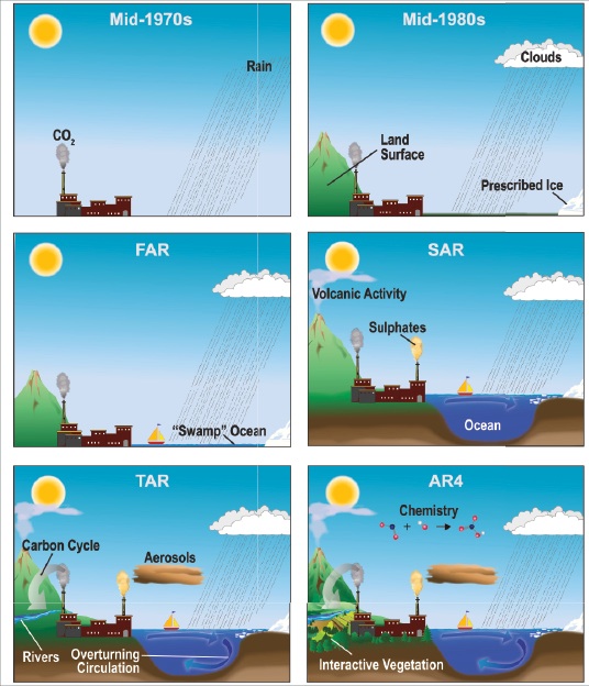
Major components of the atmosphere system such as the oceans, land surface (including soil and vegetation) and ice/snow cover, are represented by the current crop of models. The various interactions and feedbacks between these components have also been added, by using equations to represent physical, biological and chemical processes known to occur within the system. This has enabled the models to become more realistic representations of the climate system. The figure below (taken from the IPCC AR4 report, 2007) shows the evolution of these models over the last 40 years.

Climate model development over the last 40 years

Models range from the very simple to the hugely complex. For example, ‘earth system models of intermediate complexity’ (EMICs) are models consisting of relatively few components, which can be used to focus on specific features of the climate. The most complex climate models are known as ‘atmospheric-oceanic general circulation models’ (A-OGCMs) and were developed from early weather prediction models.

A-OGCMs treat the earth as a 3D grid system, made up of horizontal and vertical boxes. External influences, such as incoming solar radiation and greenhouse gas levels, are specified, and the model solves numerous equations to generate features of the climate such as temperature, rainfall and clouds. The models are run over a specified series of time-steps, and for a specified period of time.

As the processing power of computers has increased, model resolution has hugely improved, allowing grids of many million boxes, and using very small time-steps. However, A-OGCMs still have considerably more skill for projecting large-scale rather than small-scale phenomena.

IPCC model projections

As we have outlined in a previous blog, the Intergovernmental Panel for Climate Change (IPCC) developed different potential ‘emissions scenarios’ for greenhouse gases. These emissions scenarios were then input to the A-OGCM models. Combining the outputs of many different models allows the reliability of the models to be assessed. The IPCC used outputs from 23 different A-OGCMs, from 16 research groups to come to their conclusions.

Can we trust climate models?

'All models are wrong, but some are useful' George E Box 

There are sources of uncertainty in climate models. Some processes in the climate system occur on such a small scale or are so complex that they simply cannot be reproduced in the models. In these instances modellers use a simplified version of the process or estimate the overall impact of the process on the system, a procedure called ‘parameterisation’. When parameters cannot be measured, they are calibrated or ‘tuned’, which means that the parameters are optimised to produce the best simulation of real data.

These processes inevitably introduce a degree of error - this can be assessed by sensitivity studies (i.e. systematically changing the model parameters to determine the effect of a specific parameter on model output).

Other sources of potential error are less predictable or quantifiable, for example simply not knowing what the next scientific breakthrough will be, and how this will affect current models.

The IPCC AR4 report evaluated the climate models used for their projections, taking into account the limitations, errors and assumptions associated with the models, and found that:

“There is considerable confidence that AOGCMs provide credible quantitative estimates of future climate change, particularly at continental and larger scales.”

This confidence comes from the fact that the physical laws and observations that form the basis of climate models are well established, and have not been disproven, so we can be confident in the underlying science of climate models.

Additionally, the models developed and run by different research groups show essentially similar behaviour. Model inter-comparison allows robust features of the models to be identified and errors to be determined.

Models can successfully reproduce important, large-scale features of the present and recent climate, including temperature and rainfall patterns. However, it must be noted that parameter ‘tuning’ accounts for some of the skill of models in reproducing the current climate. Furthermore, models can reproduce the past climate. For example simulations of broad regional climate features of the Last Glacial Maximum (around 20,000 years ago) agree well with the data from palaeoclimate records.

Climate models have successfully forecast key climate features. For example, model projections of sea level rise and temperature produced in the IPCC Third Assessment Report (TAR - 2001) for 1990 – 2006 show good agreement with subsequent observations over that period.

So it is a question of whether the understanding of the uncertainties by the climate science community are sufficient to justify confidence in model projections, and for us to base policy on model projections. Whether we chose to accept or ignore model projections is a risk. As Professor Peter Muller (University of Hawaii) put it in an email to the Carbon Brief:

“Not doing anything about the projected climate change runs the risk that we will experience a catastrophic climate change. Spending great efforts in avoiding global warming runs the risk that we will divert precious resources to avoid a climate change that perhaps would have never happened. People differ in their assessment of these risks, depending on their values, stakes, etc. To a large extent the discussion about global warming is about these different risk assessments rather than about the fairly broad consensus of the scientific community.”

It should be noted that limits, assumptions and errors are associated with any model, for example those routinely used in aircraft or building design, and we are happy to accept the risk that those models are wrong.

For more information about climate models:

0 0

Printable Version  |  Link to this page

Comments

Prev  1  2  3  Next

Comments 51 to 100 out of 123:

  1. Oh, I found it. I posted the right equation but the wrong plot. Yours is spot on. Mine was an earlier version where I fixed the exponential periods to 1 and 50. Sorry for wasting your time. The old version is more stable, as you might expect, but still needs 60 years of data. I need to track down whether the instability is overfitting or the general problem with exponentials.
    0 0
  2. Re Kevin C #51. Glad to see we get the same results. I used the RadF.txt file from the same page as your NetF.txt file. It has the radiative forcing components broken out separately. The sum of forcings differs from your file by 0.0001 W/m2 here and there from roundoff errors. No real effect. It is interesting to compare this dataset of forcings with the ones in Hansen et al 2011 white paper. The ones used for the 1800-2003 AR4 simulations flatlined the aerosols at the 1990 levels. The Hansen whitepaper sets the sum of forcings from aerosols to be exactly -0.5 time the sum of wmGHG forcings. I'm still looking for a copy of the latest forcings from GISS, but lacking that, I'll just estimate them from the Hansen paper. ------------------------ One other thing to consider in your model is the effect of doing annual steps rather than continuous integration. A reasonable argument can be made for replacing your R(t) = 0.0434*exp(-t/1.493) + 0.0215*exp(-t/24.8) with R(t) = 0.06066*exp([-t+0.5]/1.493) + 0.02194*exp(-[t+0.5]/24.8) Where the time constant is long compared to the step (as in the 24.8 year exponential decay) the annual steps are reasonable approximation of exponential decay. But for the 1.493 year time constant, having the first coefficient of R(t) be a 1.0 isn't as good of an approximation as having the 1st coefficient be the value of R(t) at the midpoint of the year. Another way of looking at this 2 box model is that the forcings are passed through an exponential filter. The sum of the 1st 250 coefficients is 25.3023 for the 24.8 year filter, and 2.0484 for the 1.493 filter. For a continuous exponential filter, the area under the weighting curve is simply the tau. The discrete version is only 2% high for the long filter, but is 37% high for the short one. Shifting R(t) over 1/2 year makes the sum of coefficients 24.7973 and 1.46545 -- essentially equal to tau for the long filter and about 2% low for the fast one. Replacing your 0.0434 weighting factor for the short filter with 0.06066 compensates for the change in sum of filter coefficients. I haven't done the calculations, but I'm pretty sure that moving from annual to monthly calculations won't change the optimization as much if you start with R(t+0.5)as the estimate for annual response. The sum of coefficients makes for an easy test on the equilibrium sensitivity: 0.0434*2.0484 + 0.0215*25.3023 = 0.6329 C step response from 1 watt m-2. So if CO2 doubling is 3.7W m-2, the doubling sensitivity will simply be 0.6329*3.7= 2.3 C/doubling of CO2. ------------------------------------------------ Next on my agenda is to look at the correlations between various models and global anomaly time series, and then see what happens when different forcing sets are used with my emulations of the various AOGCMs. Some prelim data is that my ultra simple model using just one exponential, approximated by 6 coefficient terms, has R of 0.99 or R-squared of 0.98 with the GISS-E model. GISS-E model to GISS observed Global-Average-Temperature-Anomalies is only 0.76 r-squared. Your parameters do better than GISS with r-squared of 0.82. If the GISS observed GATA was filtered a bit, I'm pretty sure your model will come out even better in comparison to GISS-E AOGCM. IPCC suggested a 5 point filter with coefficents of 1-3-4-3-1 to reduce the year-to-year and El Nino timeframe variation. It still leaves most of the decadal variation.
    0 0
  3. scaddenp @49, You should be aware that AR1 included a paleo temperature reconstruction that Hubert Lang would have approved. The TAR showed an entirely different paleo reconstruction based on MBH 1998. In this analysis the MWP disappeared and the LIA was just a gentle dip in temperature. It was really easy for the climate models to create hindcasts that agreed with the TAR reconstruction as the temperature from 1000 A.D. to 1850 was shown as a gently falling straight line. What I am trying to tell you is that the TAR and subsequent IPCC publications demand that you ignore history. [snip] History Rools!
    0 0
    Moderator Response: [Dikran Marsupial] Moderator trolling snipped.
  4. No GC - history also show MCA occurring at different times in different places in agreement with paleoclimate reconstructions. History shows it was cold globally, especially in NH, also in agreement with paleoclimate. Where is problem there? No denial of history at all. What you falsely claim is that models cant reproduce this. I just showed you that they can. Any of them on that diagram. Still think TV trumps science? The gist of your argument I guess was that if models couldnt reproduce historical climate then there is some deep mysterious forcing at work that is miraculously going to save us. However, not so, when you have a global picture which show that you can reproduce it all from known forcings. That is not to say that there might not be something that somehow eludes our measuring systems but that is hope in the face of data. By MBH 1998 and related, can I take it you mean all paleoclimate reconstructions done since then by all groups? with all sorts of proxies. You seriously think that is a realistic position that we should respect?
    0 0
  5. GC@53 If you mean this diagram, then I rather doubt Hubert Lamb would have approved of anyone in 2011 preferring an essentially qualitative plot based on central England (rather than global) temperatures as a proxy for global paleoclimate, when there is far more global proxy data available now and 30 years more research on paleoclimate. See Appendix A of P. D. Jones et al., The Holocene 19,1 (2009) pp. 3–49, High-resolution palaeoclimatology of the last millennium: a review of current status and future prospects available here, for details.
    0 0
  6. Kevin C @51, myself @52 .. Like many things, it is obvious in hindsight. The correct expression for each R(t) coefficient is {exp(-t/tau) - exp(-[t-1]/tau} * step size. The step size in this case is 1 year, so it drops out. Since integral of exp(-x) = exp(-x), the above equation is the area of the response curve for that year. The area of R(t)becomes 1.000 using the above equation for the coefficients, since the sum of the R(t) series becomes exp(-0)-exp(-infinity)=1. This means that the scale factors for the two boxes (0.0434 and 0.0215 in your post #33) will become the equilibrium temp rise for a unit step, i.e. 0.0889 and 0.5440. This revision to the equation might help your optimizer routine, since tau would no longer affect the total equilibrium delta T.
    0 0
  7. Tom Curtis @ 43. It is not clear to me that the logarithmic incremental forcing works in reverse. The logarithmic effect is due to crowding, saturation etc.,that only apply for increases. If CO2 is the "relentless ratchet", should it not, like a ratchet, spin freely in reverse? Isn't this the reason in paleo studies CO2 is treated as "feedback only"?
    0 0
    Moderator Response: [Dikran Marsupial] The logarithmic relationship applies both for increasing and decreasing CO2, as for decreasing CO2 there is a complementary de-crowding and de-saturation etc. In paleoclimate studies CO2 is primarily treated as a feedback as the only source/sink of CO2 that counts as a forcing is volcanic emissions and changes in geological weathering due to e.g. plate tectonics. Neither of those things have a great deal of effect on climate on the timescales we are normally interested in.
  8. trunkmonkey @57, Dikran Marsupial's response is more than adequate. However, as a simple matter of logic, with a fluctuating CO2 level as has occurred over deep time, if the the relationship was not reversable, than any doubling of CO2 would bring a small increase in temperature, but halving the CO2 back to the original level would bring not bring temperatures back down to the original level. Over time, CO2 fluctuations would act as a ratchet, and in a fairly short time in geological terms you would have a runaway greenhouse. No climate scientist, however, is that alarmist - and the relationship is fully reversible.
    0 0
  9. Even climate skeptics use models but, for many, the model is simply that next year will be the same as last year. That sort of model is indeed unreliable.
    0 0
  10. PaulFP @59 "Even climate skeptics use models but, for many, the model is simply that next year will be the same as last year. That sort of model is indeed unreliable." While the snide humor may be appealing, your observation is wrong. The GISS-E model run for AR4, using the actual observed forcings for the period 1880-2003, does a poorer job of predicting the GISS global average temperature anomaly over that period than the simple "next year will be the same as last year". The GISS-E model is worse in both correlation factor and in the rms error. RMS error for both the "next year same as this year" and the GISS-E hindcast using actual forcings were around 0.15C, with the GISS-E model being slightly higher. Red is GISS-E errors vs GISS anomaly, black is "skeptic model" error.
    0 0
  11. Charlie A @60, the GISS model is not updated annually with real temperatures. Consequently to do a proper comparison with the "skeptic model" you should not provide it with that data either, ie, you should program in the initial conditions, predict 1881 temperatures from that, then predict the 1882 temperatures from the model prediction, and so on. The result will, of course, be a straight line with all temperatures predicted as equalling those of 1880 - a much worse performance than that of the GISS-E.
    0 0
  12. Charlie A@60 In addition to Tom Curtis' comment (which is spot on), the errors depicted in your graph are dominated by high-frequency annual variations, something that no model would claim to be able to predict. However, there is no long term trend in the errors, which shows that the models predict climate (which is what they do claim to be able to do) rather well. I am assuming that the GISS model E prediction is actually the mean of an ensemble of model runs (comparing the observations with a single model run would be an obviously unfair test). If this is the case, you appear ignorant of the fact that the models attempt only to predict the forced component of the climate. Whereas the observations consist of the forced component and the effects of unforced natural variability (which the averaging of the ensemble is designed to eliminate). Thus anyone with a sound understanding of what the model project means would not expect there to be a close match on a (say) sub-decadal basis, as on that timescale unforced variability dominates.
    0 0
  13. Tom Curtis @61 "The GISS model is not updated annually with real temperatures". The GISS model hindcast was updated each year with the real forcings. In fact, the GISS-E model was able to look forward into the future and know the forcings for the coming year to make the forecast for that year. The naive model of "next year same as last" didn't get to look into the future as did the GISS-E hindcast. I further handicapped the naive model by not adjusting the mean guess. For the GISS-E model, I reduced the error by adjusting the anomaly mean to match the observed mean.
    0 0
  14. Diran Marsupial @62 "the errors depicted in your graph are dominated by high-frequency annual variations, something that no model would claim to be able to predict." and "I am assuming that the GISS model E prediction is actually the mean of an ensemble of model runs (comparing the observations with a single model run would be an obviously unfair test). If this is the case, you appear ignorant of the fact that the models attempt only to predict the forced component of the climate. " The GISS-E model response is per the Hansen 2007 paper and data is available at Data.Giss:Climate Simulations for 1880-2003. These are ensembles of 5 runs, GISS-E, ocean C, Russell Ocean. My plot of this data appears to be identical to that of figure 6 of Hansen 2007. Yes, the largest component of the residuals is due to natural climate variability. However, both the naive model and GISS-E are on equal footing in regards to the effect on their errors. Do you have a better suggestion on how to test the hypothesis (or assertion) put forward by PaulFP in comment #59? His assertion is relatively straightforward: "Even climate skeptics use models but, for many, the model is simply that next year will be the same as last year. That sort of model is indeed unreliable. " In keeping with the "Can we trust models" topic of this thread, I think it is an interesting exercise to compare the performance of PaulFP/Skeptics naive model and the GISS-E model.
    0 0
  15. Charlie A, "Do you have a better suggestion on how to test the hypothesis (or assertion) put forward by PaulFP". His assertion would have the corollary that there would be no term temperature trend. This is easily tested. By comparison, the robust prediction from climate models is the 30 year trend. Climate models make no pretense of being able to predict year to year temperatures or even decade to decade temperatures with current skill.
    0 0
  16. @65 Scaddenp "His assertion would have the corollary that there would be no [long] term temperature trend." [I assume you omitted "long"] Your interpretation transforms PaulFP's statement of "Even climate skeptics use models but, for many, the model is simply that next year will be the same as last year." into the statement that the climate skeptic model is "the temperature is forever the same." If we compare the GISS-E AOGCM to a forever fixed, constant temperature, then it does indeed have some skill. If we compare GISS-E hindcast (with full knowlege of both past and future forcings) to the naive model of assuming that the yearly global average temperature will be the same as the prior year, then GISS-E loses. There is an interesting progression in model skill. My default guess for tomorrow's weather is "same as today"; but I prefer to look at a weather forecast because they have great skill in predicting weather for the next 2 or 3 days, and reasonably good skill out to a week or 10 days. For seasonal forecasts, the skill of models goes down. I assume that somewhere there has been a formal skill assessment of seasonal models done somewhere, but am not familiar with the literature. I assume, but am not positive, that seasonal forecasts have more skill than a simple naive climatological history or the Farmer's Almanac. I started reading this thread of "Can We Trust Climate Models" with the expectation that there would be a discussion regarding the assessment of skill and the testing and validation of models. Unfortunately, this most important point was omitted.
    0 0
  17. Charlie A @63, forcings are not temperatures, and nor is it an easy matter to derive temperatures from forcings alone, as the GISS-E run demonstrates. Nor where the forcings for a given year applied in determining the temperature for prior years. Consequently making use of each years annual data for the "skeptic model" does constitute a loaded test @64, yes, annual variability affects both models, but not equally. Specifically, the "skeptic model" has a negative mean (based on eyeball mk 1) from 1970 on showing that it does not predict the temperature trend. In contrast, the GISS-E model underestimates temperatures around 1910, and over estimates them in the 1940s but is otherwise superior to the "skeptic model". (If you could post a plot of the 11 year running averages it would be easier to see the relative performance over different periods.)
    0 0
  18. "Your interpretation transforms PaulFP's statement of "Even climate skeptics use models but, for many, the model is simply that next year will be the same as last year." into the statement that the climate skeptic model is "the temperature is forever the same." Well how else do you parse it? If B=A,C=B,D=C ==> A=D. For the detail on how models are really evaluated, that would be all of chapter 8, AR4, WG1
    0 0
  19. Charlie A @66:
    "I started reading this thread of "Can We Trust Climate Models" with the expectation that there would be a discussion regarding the assessment of skill and the testing and validation of models. Unfortunately, this most important point was omitted."
    Annual variability of global mean surface temperatures are in a range of +/1 0.2 degrees C per annum (approximate 90% confidence range). Atmosphere Ocean Global Circulation Models predict temperature increases of around 4 degrees C by the end of this century with Business as Usual. Frankly, it is irrelevant whether that turns out in reality to be 3.8 degrees, or 4.2. What matters is, do the models get the overall trends right given the right forcings as imputs? And if they do, what can we do to ensure forcings are not such that AOGCM's would predict such large temperature increases given those forcings? Thanks to your excercise, we now know that given a feed in of forcings, the GISS-E model predicts long term trends to a accuracy not significantly less than a 1 year lag of actual temperature data. We also know that the GISS prediction pretty much always lies within 0.2 degrees of the actual temperature. You want to quibble about that 0.2 degrees. My concern is the four degrees which you are entirely neglecting. So, we know that the models are accurate enough that they cn predict long term trends given the forcings. What then can we do to ensure forcings are not such that the models will predict 4 degree plus temperature rises remains as the only significant question.
    0 0
  20. Tom, Your uncertainty is for one year, and cannot be applied uncorrected to a century worth of data. Statiscally, when you multiple a value by ten, you multiple the uncertainty by ten also. This is slightly different in that the uncertainties are compounded, and must be treated as such. In reality, the models that predict a 4C rise by the end of the century have a much higher uncertainty than 0.2. The actual uncertainties are an order of magnitude higher; different for different models. The models are accurate based on recent temperature measurements because they have calibrated based on past observations and been fined tuned to recent values. The models are being adjusted constantly, such that by the end of century, it is entirely possible, that the models will barely resemeble those today. We can make predictions based on current knowledge of forcings, but as Hansen pointed out recently, some of that knowledge has a rather high uncertainty. This will become irrelevant if those forcings change very little, but if they change appreciably, then the unctertainties could become huge. In summary, models cannot predict short-term changes accurately due to natural variability. In the long-term, we cannot say that the models are any more accurate, as seemingly small errors today could become large errors tomorrow.
    0 0
    Moderator Response: [Dikran Marsupial] The uncertainty of a ten year trend is actually less than the uncertainty of a one year trend. The inter-annual variabilility does not apply multiplicatively to long term trends, but additively, and so the errors from year to year tend to average out to zero. That is why climatologists are interested in long term (e.g. 30 year) trends, not annual weather. Also asserting that the models are accurate because they have been fine tuned from recent observations doesn't make it true (reference required). If you look at Hansens 1988 projections, then they were actually remarkably good, and there can be no accusation of fine-tuning there (unless Hansen has a time machine).
  21. 70 - "Statiscally, when you multiple a value by ten, you multiple the uncertainty by ten also." you quite sure about that?
    0 0
  22. 70/71: sorry, re-reading, I misunderstood... scrub 71.
    0 0
  23. Model accuracy and Cross Validation I've taken my empirical lag model a little further, and I'll show some results here. But at the same time I'd like to introduce a method which scientists and statisticians in many fields use to answer the question 'can we trust our model?'. The problem here is that you can make a model which gives an arbitrarily good fit to any set of data. How? Simply add more parameters. In the extreme case, you could just tell the model the answers, giving a perfect fit. But then your model only works for the data you already have. It's also possible to do this more subtly and fool yourself into thinking you have a meaningful model when you don't. So, in the case of calculating an empirical climate response function in order to get the temperatures from the forcings, we could simply assign a value for each year in a 120 year response function. If we refine those values to get the best fit against a 120 temperature series using 120 years of forcings, we can get a perfect fit: R2=1. But the result is meaningless. R2 is not a good indicator of model reliability. A simple approach is to prescribe a minimum data/parameter ratio. For example, if we want a data/parameter ratio of at least 10, then for a 120 year time series we can use no more than 12 parameters. But this approach is limited in a number of ways, for example a noisy datum is worth rather less than an exact value. So, how do we evaluate models? For one approach to this problem, we can go back to the scientific method. We start by forming some sort of hypothesis based on the information we have. There may be multiple competing hypotheses. These hypotheses are tested when we try and use them to predict the outcome of a new observation (in Popper's terminology, we subject the hypothesis to a test which is capable of falsifying the hypothesis). Or in other words, we test the predictive power of the hypothesis. So, in the case of a climate model, we could test the model by using it to predict climate for some period in the future, and then compare it with what actually happens. Unfortunately that takes a long time. Ideally we'd like something more immediate. This is where cross-validation comes in. The idea behind cross-validation is that we hide some of our data away - often referred to as a holdout or test set, and develop our model using the rest of the data. We then use the model to predict the values of the holdout set. The quality of the model is given by the match to the holdout set, sometimes referred to as the 'skill' of the model. We can do this multiple times with multiple holdout sets if required. We could, for example, hold out one year of data, and fit a model to the rest of the data. However, there is a problem: the year-on-year temperatures are highly correlated, as Charlie and others have noted. So the prediction doesn't require much skill. So let's go to the other extreme, and set the empirical lag model a very tough challenge. We've got 124 years of data. Let's hold out 62 years, and predict the other 62. We can hold out either the first or last 62 years (or any other set) - I'll do both. The correlations only run over a few years, so this is a real test of the model. Fitting the response function with only 62 years of data is a tough challenge, I had to make some improvements. Firstly, I produced an ENSO-removed temperature series by subtracting a weighted combination of the last 9 months of SOI data from the monthly temperature data, with the weights chosen to give the best fit between the temperature data and a 61-month moving average. Then I modified the model to use a response function constructed from 5 quadratic B splines, centered at integer positions 0,1,2,3,4 on a logarithmic time axis t' where t'=ln(t+1)/ln(2.5) (i.e. at t=0,2.5,6.3,15.6,39.1), constrained such that the spline coefficients must be positive. The b-spline is a bell curve like a Gaussian, but has compact support (i.e. no long tail to infinity which we can't fit against our limited dataset). The resulting model is very marginally better than the two-box model with both time constants refined (at the cost of an extra parameter), but much more stable. Unlike the two-box model, the parameters can be fit roughly against only 62 years of data (although an 80 year training set / 40 year test would be better). Here's the results of training 3 empirical models, with the models being trained against the whole time series, the first 62 years, and the last 62 years respectively. Clearly there is some sort of predictive power here - from the early period we can make a reasonable prediction of the late period climate, and vice-versa. How can we parameterise this? Here are the R2 statistics on the whole period and the two sub-periods for each of the three models:
    R2 on 1880-2003  R2 on 1880-1941  R2 on 1942-2003  
    Fit on 1880-2003    0.8650.5000.817
    Fit on 1880-1941    0.8310.5250.774
    Fit on 1942-2003    0.8590.4820.820
    The two numbers in bold are the holdout statistics. These are the real indicators of the predictive power of the model. Note that fitting a model on only part of the data improves the fit to the included data, at the cost of making the fit to the other period (the holdout set) worse. Throwing away data makes the model worse, and the holdout statistic tells us that. Note the numbers for the early period are systematically smaller because there is less signal in that period, not because the model is necessarily worse! The values here are not absolute - rather they can be used to compare different models. So at this point we could go back and do a real test of the two-box model (if it were stable) to see whether it is a better or worse model than the b-spline model, by doing the same calculation and looking at the holdout statistics. For completeness here are the response functions for the three models: We can see the benefit of compact support in the basis functions here: The response functions reach a plateau quickly for the short-period models, and have almost plateaued in the long run model. The climate sensitivities over the limited periods are 0.58 C/(W/m2) for the full-period model and 0.41 and 0.56 C/(W/m2) for the short period models. The lower number comes from fitting the early period, where there is less climate variation to fit the model parameters. These estimates should be considered lower bounds because the model explicitly excludes any long term response beyond about a century. Question To what extent do climate modellers make use of cross-validation in the evaluation of climate models? I don't know the answer to that question. Hence my queries at #16.
    0 0
  24. Eric the Red @70, the statistical test was for the accuracy at predicting the temperature for each given year given that you have initial conditions determined for that year by the model, and that you have known forcings. The test was carried out for over a century of time. Therefore, we can be confident that with known forcings, the models make accurate predictions. They make accurate predictions even a century out, given an accurate prediction of the forcings. Now of course we cannot accurately predict the forcings a century out. But that is a little irrelevant. It is irrelevant because the predicted dominant forcing under BAU is under our control. We can continue with BAU, in which case the GHG forcings will be high enough to completely dominate the normal range of natural variability and the temperature rise will be sufficiently large that the error in the models will be of no consequence relative to that rise. Or we can keep GHG forcings at or below current levels, in which case temperatures will rise by not so much that natural variability is inconsequential, or that the error is irrelevant. The Logic is very simple. Given forcings, the model makes accurate predictions. We can't predict forcings, but we can significantly control them. Therefore the models cannot tell us what will happen, but they can tell us what will happen if we continue at BAU. Finally, with regard to your specific point, the errors introduced from year to year in the retrodictions did not compound over the century and more of the model run. That was because the results were constrained by the forcings. Hence your point is irrelevant to my point.
    0 0
  25. Tom, I agree that given accurate forcings, we can make accurate temperature predictions. Therein lies the main question: How accurate are our predictions of the forcings? Yes, we can control CO2. We can also control many other manmade factors. But, what is the normal range of natural variability? More importantly, what will be the natural response to an increase in CO2? Actually, the errors will compound. Given a climate sensitivity of 3 +/- 1.5 C/doubling, the uncertainy will increase as CO2 concentrations increase. Other forcings must also be included, although some will average out in the long term (i.e. ENSO).
    0 0
  26. Eric the Red wrote: "Other forcings must also be included, although some will average out in the long term (i.e. ENSO)." ENSO is not a climate forcing. It is a redistribution of energy within the climate. The confusion likely arises in that climate sensitivity is often estimated as a 'surface temperature anomaly'. Since ENSO involves movement of energy between the oceans and the atmosphere it can impact surface temperature anomalies on a short-term scale. This differs from a climate forcing in that it is not actually increasing the total energy in the climate system... just temporarily adjusting the proportion of that energy in one part of the climate which we commonly use as an indicator since it is (relatively) easy to measure.
    0 0
  27. Eric the Red @75: 1) The climate response to doubling CO2 is well constrained independently of the models, so the GHG component of the forcings are unlikely to be significantly in error; 2) This means the four degree plus predictions for BAU are fairly reliable; 3) Natural variability (short of catastrophic meteor impact or vulcanism) is constrained to be less than 2 degrees by the fact that mean global temperatures have remained in a 2 degree range (more probably a 1 degree range) through out the Holocene; 4) As 2 degrees is considered the upper limit for "safe" temperature increases, natural variability will not save us from the consequences of BAU (and are as likely to worsen them as to mitigate them); 5) Therefore for practical purposes, the models are reliable enough. Having said that, there is a slight possibility that increasing temperatures will reach a tripping point that will generate a significant negative feedback, thus saving our collective bacon. It is significantly less likely that it will reach a tipping point (or several of those thought to exist) which will greatly accelerate global warming. These possibilities are beyond the models (and our) capabilities to predict at the moment. For policy purposes they are irrelevant. Relying on these possibilities is like taunting Mike Tyson in the confidence he will have a heart attack before the blow drives your nose out of the back of your skull.
    0 0
  28. Eric the Red @75: "I agree that given accurate forcings, we can make accurate temperature predictions. Therein lies the main question: How accurate are our predictions of the forcings?" A main point of Hansen's recent whitepaper is that we don't know current forcings very well. The GISS-E model runs of 1880-2003 for AR4 and Hansen's 2007 paper used aerosol forcing data that was arbitrarily flatlined for the entire 13 year period of 1990-2003. In his recent whitepaper the model runs replaced that flatlined data with an approximation that set the sum of (aerosol + black carbon + indirect aerosol + snow albedo) forcings = -1/2 of (CO2 + O3 + strat. H20) forcing. I find this surprising, although it doesn't seem to have attracted much attention. People refer to tuning of model parameters, but it appears that a lot of the fitting, whether consciously or via observer bias, has been done with adjustments of the forcings.
    0 0
  29. Absolutely! Here is the problem even with cross-validated statistics. If you start tuning things to improve your holdout set statistics, then you invalidate the use of the holdout set. And yet at the same time, we want to use a holdout set to establish the validity of a model - indeed to select among competing models. All you can do is be very careful about how many decisions you make on the basis of your holdout statistics. So we come back to my questions at #16 again, which are crucial to this discussion and yet we don't have anyone who has an answer: To what extent is the response of a GCM constrained by the physics, and to what extent is it constrained by training? Similarly, the forcings that are fed into the GCMs are the result of models of a sort too. In some cases (CO2) a very simple model with ample experimental evidence. In others (aerosols) not. In the absence of a clearer understanding of the models, how do we go forward? One possibility would be to test many possible forcing scenarios against the available data. But I'm already banging my head against the limits of the instrumental record. You can bring in paleo, but the chains of inference become much longer and the data less accessible to the lay reader. (It's certainly beyond my competence.)
    0 0
  30. Charlie, It appears to be a somewhat arbitray approximation. I am not sure that it should be tied to the GHG forcigns at all, as many seem to react independently. This may have been to accommodate the large uncertainty. Kevin, I am not sure we can answer your question either individually or collectively. I think the GCMs are not constrained enough, as they tend to ignore the possibility that Tom brought up in #77; namely what are the planetary feedbacks (If any) that we be invoked when the climate changes exceeds a certain threshhold? I think you may have partly answered your question by bringing up the limits of the instrument record.
    0 0
  31. 79 Kevin C: "One possibility would be to test many possible forcing scenarios against the available data." If I understand the caption to Hansen 2011 Figure 1 correctly, the modified forcing values for 1990-2003 should be 1.3243, 0.2080, -1.3762, 0.2949, 0.9599, 1.2072, 1.2922, 1.3506, 1.4875, 1.5901, 1.6431, 1.6390, 1.6393, 1.6442 These differ from the NetF.txt values by about 0.07W/m2 in 1990, going up to a difference of 0.27W/m2 in 2003.
    0 0
  32. Eric the Red, #80 "It appears to be a somewhat arbitrary approximation. I am not sure that it should be tied to the GHG forcings at all, .." Obviously it is arbitrary to move from instrumental observations and reconstructions for the 1880-1990 period and then for the more recent 1990-2003 period change to a fixed level of aerosol forcings for the AR4 and Hansen 2007 paper. It is even more striking that four years later, Hansen changes again and decides to use the -1/2 of GHG forcing for the simulations of Hansen 2011, rather than using instrumental data. I don't know the reason for either of the changes in methodology. Do we really believe that our measurement accuracy pre-1990 was better than we have in 2011? The thread topic is "Can we trust the models?" Perhaps the real question is "can we trust the data fed into the models?" or "can we trust the data used to tune the models?" Obviously different types of emission sources have different ratios between aerosol emissions and GHG emissions. There is a lot of difference between a dirty coal plant without scrubber and burning high sulfur coal than one with scrubbers and/or using low sulfur coal. OTOH, Willis Eschenbachs simulation of the CCSM3 model resulted in 0.995 correlation with just a simple 1 box model and using only the solar, volcano, and GHG forcings. If aerosol forcings were large and uncorrelated, he could not have gotten those results. Hansen's 2001 senate testimony shows yet another version of forcings used by GISS. Note how the GHG and aerosols seem to be close to linearly related. Also of interest is the relatively low levels of aerosol forcings compared to GHG forcings. It is much less than the -0.5 factor now being used. Caption: Fig. 3: Climate forcings in the past 50 years, relative to 1950, due to six mechanisms (6). The first five forcings are based mainly on observations, with stratospheric H2O including only the source due to CH4 oxidation. GHGs include the wellmixed greenhouse gases, but not O3 and H2O. The tropospheric aerosol forcing is uncertain in both its magnitude and time dependence.
    0 0
  33. If you integrated stratospheric and tropospheric aerosols over time, how would that compare with GHG forcing? Eschenbach also stated in the reference, that "the idea of a liner connection between inputs and outputs in a comlex, multiply interconnect, chaotic system like the climate to be a risibile fantasy." He may have gotten those results by chance.
    0 0
  34. I tried a quick experiment with two choices for the reflective aerosol term. Here's the R2 values for the original forcings. I got the baselines wrong for the holdout stats, so I've redone them here. Sorry about the lack of formatting. Table rows and columns as before. 0.865 0.500 0.818 0.813 0.525 0.648 0.856 0.445 0.815 And here's the same data setting the reflective aerosol term to -0.5 * the well mixed GHG term: 0.852 0.482 0.786 0.790 0.522 0.579 0.809 0.212 0.779 Both the fitted data score (top left) and the predictive power (bold numbers) suggest this set of forcings is less good at explaining the 20th century temps using an empirical lag model. (But fitting on only 62 years of data is probably unrealistic. Should really run with 31/93, 93/31, and maybe 31/62/31 predicting the middle.) Eric: According to my (possibly flawed) understanding, Eschenbach's 'risibile fantasy' quote is hard to reconcile with the physics of the system. Radiative forcing is simply a measure of the extra energy being pumped into the system. Of course it is simply related to how the energy in the system varies over time. The only reason this isn't transparently obvious is that we don't have a simple way to measure that energy - we only measure the temperature of a subset of the components, which in turn have different heat capacities and are continuously exchanging energy among themselves. Thus, although there are annual variations, I think it is totally reasonable that the global temperature averages of the GCMs can be modelled with a simple lag model - and clearly so does Hansen, since he does exactly that in his 2011 draft paper. Eschenbach's other mistake is that his model is too simple. His single time constant can't reflect the more complex response function of the real system. This would be OK apart from the volcanoes, which are the only forcing with sharp discontinuities. As a result he has to fudge the volcanic forcing. (This was Tamino's point, but my alternative model parameterisation supports his conclusion.)
    0 0
  35. Thanks Kevin, I am keenly interested in the aerosol research, and hope to see much more in the near future. Especially given the high uncertainties attributed to aerosols and clouds. Volcanoes have always been difficult to model for endless reasons. BTW, if you like simplicity, take the monthly CRU data starting from 1880 and subtract a trebnd equal to 0.005C/month (0.6C/century).
    0 0
  36. And here are the results with the original forcings to 1990, and Hansen's 2011 values from Charlie's post #81. (Misread Hansen first time, sorry). 0.861 0.491 0.808 0.792 0.525 0.584 0.817 0.194 0.811 Still worse.
    0 0
  37. Kevin C @84. "Eschenbach's other mistake is that his model is too simple. His single time constant can't reflect the more complex response function of the real system." His simple single time constant lag model has 0.99+ correlation with the output of two different AOGCMs. Like you, he doesn't believe this is likely to be a good replica of the real, complex response fuction of the real climate system. That was the point of that series of articles. He was surprised at well the GCM model outputs (on a global average) could be replicated by simply multiplying the forcings by a constant, or multiplying by a constant and then a lowpass filter. The models parameterize things like clouds. So the models wouldn't show things like a change in the daily cloud patten so common in the tropics. Clear in the morning, clouding up and raining in early afternoon. It wouldn't take much of a time shift in the daily pattern to have a large, relatively fast feedback.
    0 0
  38. Kevin C, you may find the following article from International Journal of Forecasting interesting as it uses a variety of metrics to compare the HadCM3 AOGCM of Hadley center with some time series forecasts. Validation and forecasting accuracy in models of climate change Non-paywalled draft paper Discussion and additional info from author at Pielke Sr's blog. When looked at from the point of view of a statistician or forecaster, the climate models don't do very well globally, and are very poor at regional predictions. The climate models, in many tests, have predictive capability worse than a random walk.
    0 0
  39. Charlie A thanks for pointing us to this very interesting paper. Though, you fail to put the paper in the right context and come to clearly wrong conclusions. The paper is about decadal forecasts, as opposed to long term (climatic) projections. I'm sure you agree that it's a completely different issue. So, when you say that "the climate models don't do very well globally" you should use the singular, given that they use just one decadal forecast climate model (DePrSys), and specify the time span. Indeed, on going from t+1-t+4 years to t+10 years things change drammatically (table 8); DePrSys proves to be, not the best, but a good one. Your last sentence is also incorrect. Indeed (fig. 4) random walk is better than any model in the time interval where there's no trend and "From around 1970 there is a clear preference for models that are able to model trend and the ratio turns against the random walk". This should come as no surprise to anyone who knows what a random walk is and that there's not just CO2. Regional forecasts are more problematic. Though, the paper compares the data from six spots to DePrSys. Here small scale influences, beyond the resolution of the model, are likely do be an important factor. In my opinion, the comparison should have been done on the medium scale appropiate to the resolution of the model. You linked to Pielke Sr. without comments, so this final remark is referred more to him than to you. Quote mining is easy and usually I avoid it because I think that science is more interesting, let alone important. The following quote (but could have been more) from the paper should be considered an exception to my own rule: "But there is no comfort for those who reject the whole notion of global warming– the [statistical] forecasts still remain inexorably upward with forecasts that are comparable to those produced by the models used by the IPCC."
    0 0
  40. I hope this statement below meets the criteria for this particular thread. If not, let me know if there is another place where I might share it with readers. John Nicol It is interesting to read the IPCC report, in particular Chapter 8 and then to read the many interpretations which are evident here. In its final analysis in AR4, the IPCC stated that amny of the parameters which it could include as input to the models were very uncertain. There were also many variables and behaviours which were poorly understood. In the model's outputs they conceded that precipitation, clouds, convection and several other very important features which have very strong influences on weather and by definition on climate - since climate is simply the average of "weather" taken over thirty years" (an internationally accepted definition of climate). The one crowning statement from the IPCC AR4 is that "In spite of these uncertainties, we have a high level of confidence in the assessment of the temperature." - or words to that effect. It is also stated in that document that the temperatures calculated from each of the models, for doubling carbon dioxide, range from approximately 1 to 5 degrees, after eliminating ,models whose results were, in the words of the IPCC, "implausible" which is code for "returned negative values for the temperature increase on doubling CO2". If a finding of +1 is plausible while below another implausible finding of magnitude +5, why is another with its value 4 less than +1 i.e. of -3 considered implausible? After all, according to the results shown in Chapter 8, no two of the 23 models shared a similar result! I have some difficulty understanding the rationale behind these fairly arbitrary conclusions in what is, at least ostensibly, an effort to determine scientifically what will be the effect of doubling carbon dioxide. There are no references in the IPCC report which show independently that carbon dioxide causes warming. It is "remonstrated" only in the results of the models. (-Snip-) As with all science, the above analysis may be incorrect but it is thrown in to stimulate discussion about the role played by Carbon Dioxide in the atmosphere. I look forward to reading comments and criticisms which provide a different approach to the problem.
    0 0
    Response:

    [DB] Apologies, as you must have spent substantial time and effort developing and posting your comment, but the snipped majority falls outside the scope of this thread. 

    As dana1981 points out, you are welcome to break up your longer comment into components and post those on more appropriate threads for others to read & discuss if you wish (the Search function will find ample threads; select the most appropriate for the comments).

    Alternatively, you could post the entire comment as a blog post on your own blog and then provide a link here for interested parties to follow.

  41. John Nicol @90, if I where a moderator here, I would delete your post. This is not because there is nothing worth discussing, or worth avoiding discussing in your post. It is because any response in detail to any but the second and third paragraphs in the post would be immediately off topic in this thread. The onus should be on you to find the appropriate topic for that detailed discussion, post the relevant logical points of your essay at those locations, and then link back to those discussion here, with a brief comment on the relevance to the topic here, the reliability of models. By avoiding that onus, it appears that you want to make your detailed claims but use the comments policy to shield yourself from detailed criticism. As I am sure that is not what you want to do, perhaps you could do the moderators a favour by reposting the relevant sections of the above essay in the appropriate topics, and restricting the discussion here only to factors directly bearing on the reliability of models. Of course, you may not want to do the moderators any favours by so doing - but then why should they do you favours by carefully snipping only those sections of topic here rather than simply deleting the whole post?
    0 0
  42. John Nicol, if you want to dispute the existence of the greenhouse effect, there are posts on that subject. If you want to discuss climate sensitivity, there are posts on that subject as well. It becomes impossible to respond to you when you dispute so many scientific topics in one comment, which is why we have the 'no off topic comments' rule. I will say that no climate models have negative values of climate sensitivity within their possible range, so I think it's quite obvious why they're considered implausible, aside from the rather obvious physical reasons [i.e. negative sensitivity would prevent transitions from glacial to interglacial periods]. Butl that's an issue that should be discussed in the climate sensitivity post comments. Please make use of the search bar.
    0 0
  43. Riccardo #89 "The paper is about decadal forecasts, as opposed to long term (climatic) projections. I'm sure you agree that it's a completely different issue." Are you saying that we should not trust the climate models to make reliable decadal projections? The main article says "For example, model projections of sea level rise and temperature produced in the IPCC Third Assessment Report (TAR - 2001) for 1990 – 2006 show good agreement with subsequent observations over that period." Riccardo -- do you feel this is an inappropriate statement? It seems to me that the main article claims that short term projections are reliable. Do you disagree? The link provided in the main article in that section is to Rahmstorf 2007, which looks compares the 2001 TAR projections to the global average temperature observations through 2006 and, through the use of an innovative method of handling end point data extension, finds that the models underestimate the actual trend. Of course, later observations have shown that the Rahmstorm method of smoothing and extending data is faulty, but that is the article chosen by Verity to support the statement that the 2001 TAR projections through 2006 are good.
    0 0
  44. Charlie A "When looked at from the point of view of a statistician or forecaster, the climate models don't do very well globally, and are very poor at regional predictions. The climate models, in many tests, have predictive capability worse than a random walk." (emph. mine) This is your interpretation of the paper, not mine.
    0 0
  45. Again thanks to the moderator [DB] for your comments and invitation to include links. I was previously of the impression that it might be inappropriate to give another reference link for people on your post as a lot of other sites disallow the invitation to their own "audience" to go elsewhere. However, if that is OK here it would certainly make it easier perhaps to keep everyone happy and prevent unsettling other guests. Best, John
    0 0
  46. I thought I had included a comment apologising to Dana and Tom Curtis for upsetting them with my comments, but don't see it now. Briefly this time: Sorry, I will be careful as to what threads I post to. Best wishes to you both, John
    0 0
  47. Charlie A @ 93. "Are you saying that we should not trust the climate models to make reliable decadal projections?" I think the answer is yes, that is what he is saying. It is a point that is well established on various threads here and mentioned earlier in this thread that the models are only good for a 30 year trend. This is largely because they are unable to predict the only quasi periodic alphabet soup of ocean atmospheric oscillations (PDO etc., I like to call the O's)These oscillations are able to tap into an enormous pool of ancient bottom water that like the loose end of a fire hose swings to alternate sides of the ocean basins. As CB Dunkerson points out all of this is just redistributed energy, but so are the obliquity and precessional Milankovitch influences. There is a thousand year supply of this cold water to frustrate decadal scale predictions until these oscillations are sucessfully modelled. This is why Hansen (et al 2011)has joined a growing chorous including Kevin C saying hey, if all you get is a 30yr GMAT trend line, I can do that on a spreadsheet.
    0 0
  48. Charlie @87:
    His simple single time constant lag model has 0.99+ correlation with the output of two different AOGCMs. Like you, he doesn't believe this is likely to be a good replica of the real, complex response fuction of the real climate system. That was the point of that series of articles. He was surprised at well the GCM model outputs (on a global average) could be replicated by simply multiplying the forcings by a constant, or multiplying by a constant and then a lowpass filter.
    Sorry, I must have mis-expressed myself. That is not my position at all. I think it is completely unsurprising, indeed inevitable, that a lag-model of some sort will duplicate the behaviour of both models and the temperature record. Why? Because conservation of energy trumps chaos. So I think Eschenbach surprise springs from a failure to go back to the physics. My comment about the model being too simple applied to his single-box model only, and the resulting need to adjust the forcings, not to lag models in general. The only question is over what time scale conservation of energy trumps chaos. Clearly averaging over the globe, a year, and an ensemble of model runs is plenty (hence my correlation to the ModelE ensemble is 99.3%, haven't tried CCSM). It would be interesting to compare against individual runs to get an idea of the range of variation, and see if that compares to the variation in the real temperature series. My understanding is that much of the remaining variation arises from energy 'sloshing about' inside the system, coupled with the facts that we only observe a tiny part of that system and that we look at temperature not energy.
    0 0
  49. Charlie A wrote "Are you saying that we should not trust the climate models to make reliable decadal projections?" I think the point that Riccardo was making is that the accuracy of decadal predictions is not necessarily a useful indicator of the ability to make reliable projections on the centential time scale that is relevant to any polity decision. The Fildes and Kourentzes paper is deeply flawed because it tries to cast doubt on the IPCC use of model based predictions on the grounds that statistical methods make better decadal predictions. This is a non-sequitur, the conclusion is not justified by the premise. On a decadal scale, the observations are dominated by sources of natural variability such as ENSO. This is the reason why claims like "no global warming since 1998" are bogus. Decadal observations tell you very little about forced climate change. Thus statistical methods are as good as anything for decadal predictions. Now climate models do not attempt to directly predict the observed climate, they attempt to estimate only the forced component. The ensemble mean is a prediction of the forced change, the error bars (formed by the spread of the ensemble predictions) is an indication of what climate change we are likely to actually observe (taking natural variability and other uncertainties into account). On a short timescale (e.g. decadal), the effects of forced climate change are small compared to natural variability, so one should expect the forced climate change to be different from the observations. However on a decadal scale the error bars will be very wide, so the models are still reliable (as they tell you how uncertain their prediction is). GCM predictions of decadal climate are reliable, provided you bear in mind that it is something they are not really intended for, and you take into account the error bars. Essentially decadal predictions are long timescale weather prediction, not climate projection.
    0 0
  50. Dikran Marsupial I'm not even sure that the paper's conclusions are flawed. They might be ambiguos when they do not explictly say that they're talking about decadal forecasts. Here I see more of a misinterpretation than a flaw, given that the authors consider a decade as the policy relevant time range; I disagree on this, but the authors explicitly express their point of view in the paper. The authors also note that on longer time scales GCM do a good job, as I quoted in a previous comment. I think that this paper is a contribution to the understanding of the weaknesses of the DePrSys GCM (and probably of any GCM) when modified to try decadal projections. If I understand correctly what they say, their suggestion is to re-initialize the GCM each year with the measured status of the climate system, one thing that current GCMs don't do by construction. This might be a good way to improve GCMs when dealing with decadal projections, but it doesn't have much to do with long term climatic trends. A general point on the noise skeptics are making. Why should I be surprised if an athlete trained to run a marathon runs 100 m and doesn't win?
    0 0

Prev  1  2  3  Next

You need to be logged in to post a comment. Login via the left margin or if you're new, register here.


The Consensus Project Website

THE ESCALATOR

(free to republish)


© Copyright 2024 John Cook
Home | Translations | About Us | Privacy | Contact Us