


 Arguments


Recent Comments
Prev 1160 1161 1162 1163 1164 1165 1166 1167 1168 1169 1170 1171 1172 1173 1174 1175 Next
Comments 58351 to 58400:
-
Tom Curtis at 09:11 AM on 27 May 2012Dead Ahead: Less Rainfall for Drought-Sensitive Southern Hemisphere Regions?
bath_ed @2, I am no expert, but my understanding is that semi-arid regions still retain soil, ie, fine grained dirt including some humus, which can be the basis of agriculture with more water. Even then, many semi-arid soils are poor quality, and will quickly become exhausted with ordinary agricultural practices. In contrast, in truly arid areas, the dirt often consists of coarse sands, or is salty, or covered in rocks; and will require substantial preparation to be suitable for agriculture. Consequently, I would expect expansion of the Intertropical Convergence Zone into the Sahel would give an immediate boost to agriculture, but expansion into the Sahara would not. -
bath_ed at 07:18 AM on 27 May 2012Dead Ahead: Less Rainfall for Drought-Sensitive Southern Hemisphere Regions?
A minor nitpick but it is Verlorenvlei (often also spelt Verlorevlei) not Lake Verlorenvlei. Vlei is an Afrikaans word derived from the Dutch vallei (valley) with a meaning that has shifted to mean a marsh, lake or other wetland, and is widely used in (South African) English. I'm not sure about lack of soils for irrigation - I believed that many arid and semi-arid lands provided good crops if provided with artificial irrigation. -
Bob Lacatena at 04:35 AM on 27 May 2012The human fingerprint in the seasons
SRJ, Actually, I'll backpedal a little, in that the basic argument that winter will see more nighttime warming, and that is due to at least in part to radiative effects, is true. But... 1) All warming, regardless of cause, will invoke a strong, positive water vapor effect which will demonstrate this effect. 2) Any effects are complicated by everything else going on (as I already stated). 3) The implementation of Modtran you are using is ill-suited to this in particular because it is not simulating night-time, or an entire day or month or season. It is not a "climate model." It is a simple calculation that says, at some moment in time, given certain conditions, what will the radiative profile look like. [In fact, I'm now wondering what "time of day" that particular program is using -- I assume noon -- because that obviously is a factor as well. I'm surprised it's not another parameter to be selected.] The main point you should take away from this is that Modtran is absolutely the wrong tool for the job in this case (as far as I can tell). -
SRJ at 02:30 AM on 27 May 2012The human fingerprint in the seasons
# 174 Sphaerica Thank you for the response. But if it is as you say that increased winter warming is not a direct result of radiative effects, then I think the opening section of this article is too simplifying. But I guess that is how it is to avoid it being to technical. I think I will have to read Arrhenius' article to get a better understanding of this. -
jyyh at 00:35 AM on 27 May 2012Arctic Winter Analysis
Now how did the embedding of the images go... Took one section of the Modis Rapid Response site (in between Beaufort Sea and East Siberian Sea) and enhanced contrast as to see if the different thicknesses of ice could show up, as the melt progresses the ice turns a bit grey (albedo decreases) so this method could give some indication of the health of the icepack...: judgement: not very healthy.
-
jyyh at 20:46 PM on 26 May 2012Dead Ahead: Less Rainfall for Drought-Sensitive Southern Hemisphere Regions?
OTOH, the expansion of Hadley cells as the evaporation in the tropical oceans increases could make the rainy season of tropics occur more widely and for a longer period. But as this expansion would occur on locations that are currently deserts there would be no more soils for irrigation. Speedy check on the map would indicate that movement of 1200km (~width of the subtropical desert belt) would be required to continue farming on these locations. In the Northern Hemisphere things could change quicker as the polar cell will be destroyed by the abolition of Arctic ice at least in summer. And is the Hadley circulation constrained by the tilt of the Earth, so it cannot expand so much? Some sort of simple model might be enough to answer this question, as these are large-scale structures of the atmosphere that are shifting locations. -
Philippe Chantreau at 15:35 PM on 26 May 2012Mars is warming
Thank you Tom, this is the point I was trying to convey in post #11 up there a few years ago. Intellectual bankruptcy is the word indeed. -
Tom Curtis at 12:00 PM on 26 May 2012Mars is warming
I'm a bit bored, so I've decided to actually show the "big beautifol really obvious ice caps" Duncan claims to have seen in the 70's. First from the Mariner missions in 1969: The two images where taken be separate craft on flybys, within six days of each other in 1969.
Then from the Viking program in 1980:
The two images where taken be separate craft on flybys, within six days of each other in 1969.
Then from the Viking program in 1980:
 Viking even produced a mosaic map of Mars, showing the massive polar ice caps that existed just 30 years ago:
 If you think I am laughing at the intellectual bankruptcy of deniers like Nahle who try to flog this dead horse, you are right.
-
muoncounter at 11:03 AM on 26 May 2012Mars is warming
Scott Duncan #28: "pathetic small and mostly non-existent ice caps." This is really big news, or at least it was in 2003: Mars is melting Like Earth, Mars has seasons that cause its polar caps to wax and wane. "It's late spring at the south pole of Mars," says planetary scientist Dave Smith of the Goddard Space Flight Center. "The polar cap is receding because the springtime sun is shining on it." The south pole is indeed more dynamic: The coincidence of aphelion with northern summer solstice means that the climate in the northern hemisphere is more temperate than in the southern hemisphere. In the south, summers are hot and quick, winters long and cold. Seasons! Who'd have thought that? -
Tom Curtis at 10:13 AM on 26 May 2012Richard Alley's Air Force Ostrich
You can find the full list of the "How to talk to an ostrich" videos here: http://earththeoperatorsmanual.com/main-video/how-to-talk-to-an-ostrich It is only one of the resources associated with Richard Alley's book, Earth the Operator's Manual, and associated PBS series. Other interesting resources are the ETOM "heroes"; and a series of articles about the issues related to global warming. -
Tom Curtis at 09:10 AM on 26 May 2012Mars is warming
Well, let's look at the photos, or images at least: Mars, 1873: Mars, 2007:
 So from 1873 to 2007, Mar's NH polar cap has approximately the same size, while its SH polar cap has greatly expanded.
But what about images like this:
So from 1873 to 2007, Mar's NH polar cap has approximately the same size, while its SH polar cap has greatly expanded.
But what about images like this:
 According to AGW denier, Nasif Nahle, this is a ...
"Sequence of photos illustrating the Global Warming on Mars. Observe how Mars' Polar Caps have been melting since 1990, the same phenomenon has been occurring on Earth."
Except, when I look at the pictures, I see the large expansion of the SH polar cap from 1995-2001, followed by its contraction. I also see the initial contraction of the NH polar cap, followed by its expansion, after which it is hard to say what it does because it is hidden behind the limb of the planet. Clearly, the polar caps of Mars are very dynamic. The rapidity with which they change their extent can be seen in this montage showing the NH cap over a period of six months: As we know, by 2001,it had already regained its lost extent, and no doubt lost it again before regaining it in 2007.
AGW deniers, like Nahle, are attempting to portray images of seasonal variation as proof of global warming on Mars. But if you look at all the evidence, its easy to see through their parlour trick.
As we know, by 2001,it had already regained its lost extent, and no doubt lost it again before regaining it in 2007.
AGW deniers, like Nahle, are attempting to portray images of seasonal variation as proof of global warming on Mars. But if you look at all the evidence, its easy to see through their parlour trick.
-
Scott Duncan at 07:48 AM on 26 May 2012Mars is warming
Interesting thread people. But one slight problem - I have been watching Mars since a young lad in the Apollo moon landings. Look at the photos of Mars in the 1970's - big beautifol really obvious ice caps. Now look at Mars - pathetic small and mostly non-existent ice caps. Why? [snip]Moderator Response: [Dikran Marsupial] Off-topic gish gallop snipped. Please familiarise yourself with the comments policy. SkS is for scientific discussion, not rhetorical debate. Data and references to scientific litterature that support your assertions are always much more convincing than anecdotal evidence. -
Bob Lacatena at 06:27 AM on 26 May 2012The human fingerprint in the seasons
173, SRJ, I think there are a number of things you are doing wrong... for example, I think you should start by balancing your scenarios with the outgoing, top of atmosphere radiation equal to an appropriate, incoming (solar) annual/daily average. But right there you run into a big problem, because the daily average for the planet (239 W/m2) varies dramatically by latitude and season. More importantly, there are many, many hugely important factors that are not modeled in pure radiative transfer (such as convection, clouds, water vapor, and albedo changes due to changes in snow and ice). The largest is the convective transport of heat and moisture not only upward, but also poleward. A noticeable increase in temperature/heat at the equator will translate into additional (and further) transport of heat/moisture north and south, in addition to radiative warming at those locations. The point is... increased winter warming is not a direct result of purely radiative effects of increased greenhouse gases. It is instead a result of the multiple confounding factors in climate, and one that is predicted by (a) complex climate models that simulate those factors and (b) paleo-studies that find such differences in past climate change events. -
Composer99 at 01:44 AM on 26 May 2012The 5 characteristics of scientific denialism
IMO there are two additional characteristics of scientific denialism which do not necessarily fit in the characteristics described here in the OP or over at Denialism blog: Misrepresentation: Denialists tend to misrepresent - whether ignorantly, inadvertently, or intentionally - the scientific literature as well as the statements and positions of scientists, scientific bodies, and other advocates (individuals or groups) supporting the mainstream/consensus position. Such misrepresentations are made in the service of almost every other characteristic of denialism, which is why I would promote them to a separate characteristic. Examples: - misrepresentation of the content of the hacked UEA-CRU emails is undertaken to reinforce the accusations of conspiracy/hoax/what-have-you - misrepresentation of credentials is used by denialists to reinforce their acceptance of fake experts (e.g. Monckton's claims regarding the House of Lords or the Nobel prize) - cherry-picked papers are often misrepresented as stating some conclusion not related to, or out of line from, or even in diametric opposition to, what they actually say (e.g. the recent paper regarding Medieval Climate Anomaly at Antarctic sites, Monckton on Greenland ice, Forbes magazine's blowing Spencer & Braswell 2011 out of proportion) - the misrepresentation of climate science's basis being solely dependent on models is a necessity for setting up impossible expectations/shifting goalposts, as is the misrepresentation of historical denialism (e.g. claims that "skeptics" have never denied warming, or that CO2 causes warming, or the like) - most obviously, misrepresentations are often crucial components of typical logical fallacies such as ad hominem arguments, appeals to emotion, false equivalencies, and straw men arguments - related to my other suggested characteristic, below, the continuous use of misrepresentation creates an environment in which denialist claims can be accepted with undue credulity. Credulity: Denialists tend to accept - and propagate - with unseeming credulousness claims made against the body of mainstream climate science, or against scientists or advocates espousing mainstream climate science, or even against the physics underpinning mainstream climate science. Such credulity extends to accepting claims made on the basis of poor physics (e.g the typical crank claim that the atmospheric heat-trapping effect violates the laws of thermodynamics or other stuff routinely discussed @ Science of Doom), poor statistics (e.g. the material routinely debunked by Tamino), long-ago-refuted or dismissed material (e.g. claims that the heat-trapping effect of CO2 is saturated) or even self-contradicting sets of claims (as documented elsewhere here on Skeptical Science. As with misrepresentation, credulity is such a key component of other characteristics of denialism that IMO it deserves to be a characteristic of its own. Also, suffice to say, the credulity required to engage in denialism puts paid to the self-identification of denialists and contrarians as reasonable skeptics. Examples: - Many claims of conspiracy (such as suggesting peer review == theocracy, or claiming the resignation of the editor-in-chief of Remote Sensing over Spencer & Braswell 2011 was evidence of the IPCC 'clique' at work) require a rather credulous mindset - indeed, accepting the existence of a vast conspiracy comprising thousands of scientists across the world, the IPCC, every major scientific academy and almost every major scientific organization requires a very credulous mindset - I submit that it takes a great deal of credulity to accept the likes of Anthony Watts, Christopher Monckton, or Fred Singer, as superior authorities to the IPCC, the NAS, and notable climate scientists - Since most cherry-picking is obvious once the cherry-picked source or information is examined on its own terms or in reference to the literature, some degree of credulity is required to accept cherry-picked claims without further investigation (which is what the cherry-pickers are hoping for, of course) - Accepting that climate science must meet unachievable hurdles of evidentiary support before informing policy, compelling action, or being accepted as "real" science, when compared to the evidentiary support it actually has or compared to the evidentiary support for other scientific disciplines which inform policy-making or personal/societal action, again, requires credulity - Creduility required to accept fallacious logical arguments? Check - With regards to the additional characteristic suggested above, denialist credulity in climate science allows the unquestioned acceptance of various misrepresentations, however blatant. -
dana1981 at 00:52 AM on 26 May 2012Modeled and Observed Ocean Heat Content - Is There a Discrepancy?
Note from the first graphic showed by Tom @11, there is not a significant divergence between GISS-ER and Lyman (2010). I prefer looking at the trends rather than the graphs, because as Tisdale and Evans showed, improper baselining can lead to a very wrong conclusion when relying solely on graphs, or just on one piece of data, i.e. Levitus 0-700m. -
Tom Curtis at 22:48 PM on 25 May 2012Modeled and Observed Ocean Heat Content - Is There a Discrepancy?
Muoncounter, the "large departure" is a feature of the 0-2000 m data, only of the 0-700 m data. It is, as you note, a short term feature and probably related to the hiatus which follows it, and which Dana discusses in the OP. As to sliding the model observations across to match it - the 0-700 m data and 0-750 meters model predictions do have a common baseline which is displayed in the graph. Therefore it would be incorrect, IMO, to readjust the model prediction to show a better fit. The divergence between the 0-750 m model data, and 0-700 observed data is a genuine divergence in need of explanation. Much of that explanation has, of course, been provided by Meehl et al. -
muoncounter at 22:11 PM on 25 May 2012Modeled and Observed Ocean Heat Content - Is There a Discrepancy?
Tom, Your curve-sliding exercise is nice, but why not take this tack? What is the origin of the large departure of data from models which appears to occur in 2001-2002? This short-term 'event' is clearly not a part of the models. If the model runs are offset to include it, they're back in better alignment with the data. It is a lot like saying that we cannot predict the date and severity of an explosive eruption. We know they will happen, just not where and when - and so they cannot be expected to occur on schedule in a forecasting model. -
SRJ at 21:51 PM on 25 May 2012The human fingerprint in the seasons
I have tried to use Modtran to illustrate the fact that winters should warm more than summers. But I cannot get it right. Here is how I do it: - first I calculate the intensity of outgoing long wave radiation I_out for an atmosphere without CO2 for "Localilty" choosen as "Mid lattitude summer". - Then I increase the CO2 concentration to 1000 ppm and adjust the offset for T_ground until I_out matches the value without CO2, since that means the steady state is reached once again. For "Mid lattitude summer" I get the offset for Tground to 9.25 K. Doing the same for "Mid Lattitude Winter" I get the offset to be 8.02 K. That means more warming in summer than in winter. Can anyone explain what I am doing wrong and how to correctly illustrate the effect that increasing GHG's leads to winters warming more than summers using Modtran? Is the problem that Modtran is too simple to this? -
Kevin C at 20:35 PM on 25 May 2012Modeled and Observed Ocean Heat Content - Is There a Discrepancy?
Ah, I think From Peru@12 and Tom@13 have nailed it! I was also seeing FP's shocking divergence, but FP correctly observes that for energy imbalance we are only interested in the gradient. Which Tom then shows by offsetting the 0-2000m curve in #13. -
Tom Curtis at 19:48 PM on 25 May 2012Modeled and Observed Ocean Heat Content - Is There a Discrepancy?
From Peru @12, I see that Bob Tisdale does in fact have the updated graph, which is no being displayed at Real Climate as well: Again, I do not see a "shocking divergence" in the curves. Consider solely the 0-2000 m data, to eliminate any issues with the divergence. Below I have placed a copy of that data so as to overlay the whole ocean model prediction:
 As you can see, when so overlaid, there is little divergence between them. The trend of the OHC data will be very similar the model prediction, something we already knew from the data cited by Dana. The large apparent divergence in the graph is simply the product of a small divergence in slope carried forward for a significant period.
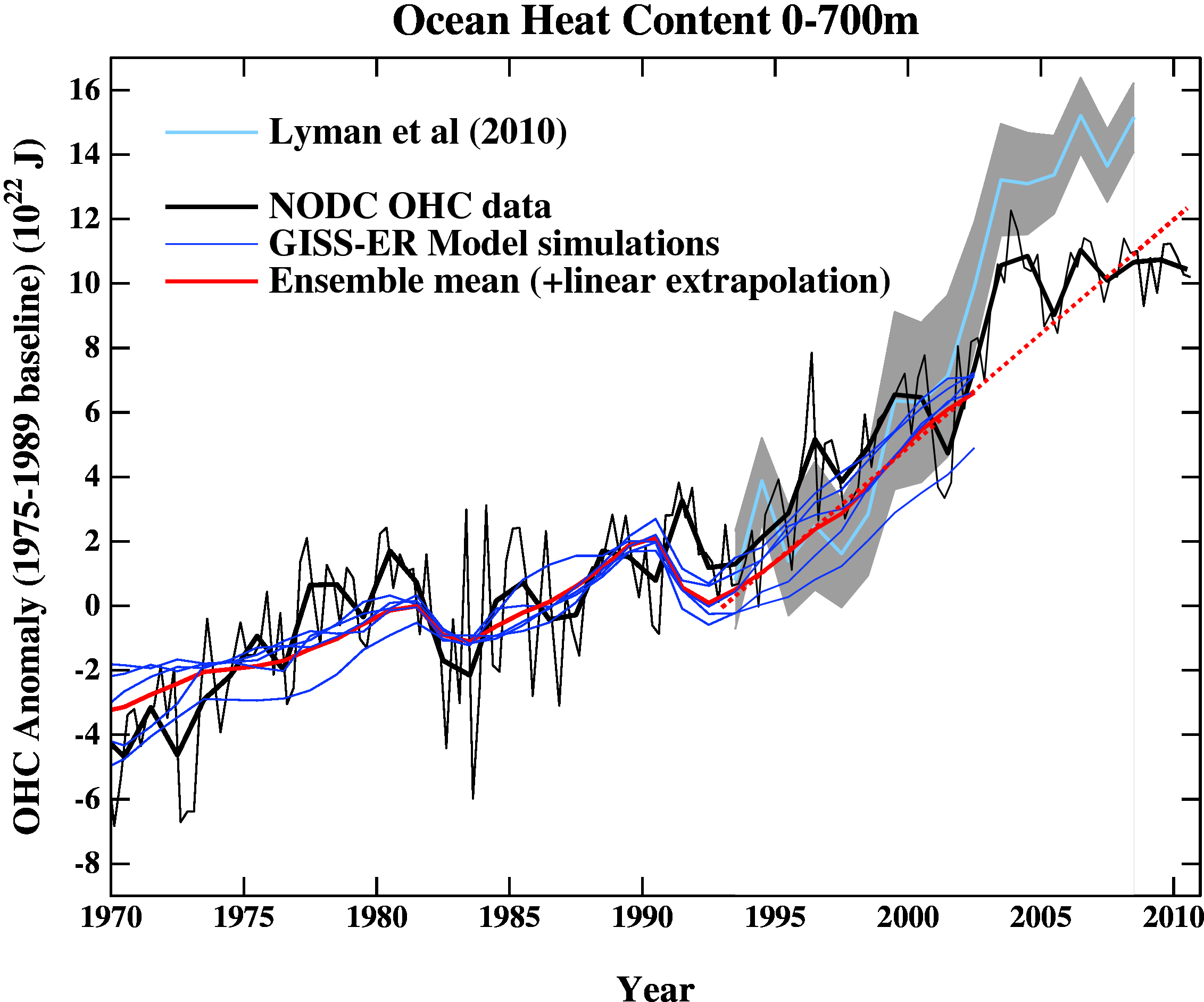
By comparing the prediction and data over just the interval 2000-2010 while using a baseline from 1975-1989, we effectively add each divergence from 1982 (the baseline midpoint) to 2000 to the divergence over the period from 2000-2010, thus exaggerating it. If we wanted to compare the trend over the entire period, we should baseline the observed data over the entire period as well. If we to do so, much of the separation between prediction and observation would disappear. This is because the observed 0-2000 m OHC would follow a steeper slope than the 0-700 m OHC from the baseline period:
As you can see, when so overlaid, there is little divergence between them. The trend of the OHC data will be very similar the model prediction, something we already knew from the data cited by Dana. The large apparent divergence in the graph is simply the product of a small divergence in slope carried forward for a significant period.
By comparing the prediction and data over just the interval 2000-2010 while using a baseline from 1975-1989, we effectively add each divergence from 1982 (the baseline midpoint) to 2000 to the divergence over the period from 2000-2010, thus exaggerating it. If we wanted to compare the trend over the entire period, we should baseline the observed data over the entire period as well. If we to do so, much of the separation between prediction and observation would disappear. This is because the observed 0-2000 m OHC would follow a steeper slope than the 0-700 m OHC from the baseline period:
 So far as I can see, once we use a correct base lining, the divergence issues become the minor issues discussed already by Dana. Of course, Tisdale will continue to use incorrect baselines, and not discuss the full range of observational data sets and model results because, quite frankly, he can't afford to allow his blind men to access more than just a trunk, or a leg, or a tail, lest they realize recognize the elephant of global warming in the data.
 Moderator Response: TC: HTML edited to show correct first image.
 -
hengistmcstone at 17:05 PM on 25 May 2012Skeptical Science now an Android app
Hi, the link on the right to the Nokia App just takes me to Nokia 'this product is no longer available'. I was wondering if that was a glitch or whether it has been withdrawn? Any chance its being revised and will become available again? Just bought a Nokia. -
Asteroid Miner at 15:32 PM on 25 May 2012The True Cost of Coal Power
http://www.ornl.gov/info/ornlreview/rev26-34/text/colmain.html Coal contains: (snip) and all of the decay products of uranium, (snip), Antimony, Cobalt, Nickel, Copper, Selenium, Barium, Fluorine, Silver, Beryllium, Iron, Sulfur, Boron, Titanium, Cadmium, Magnesium, (snip), Calcium, Manganese, Vanadium, Chlorine, Aluminum, Chromium, Molybdenum and Zinc. There is so much of these elements in coal that cinders and coal smoke are actually valuable ores. We should be able to get (snip). Unburned Coal and crude oil also contain (snip). We could get all of our uranium and thorium from coal ashes and cinders. The carbon content of coal ranges from 96% down to 25%, the remainder being rock of various kinds. If you are an underground coal miner, you may be in violation of the rules for radiation workers. The uranium decay chain includes the radioactive gas (snip), which you are breathing. Radon decays in about a day into polonium, the super-poison. Chinese industrial grade coal is sometimes stolen by peasants for cooking. The result is that the whole family dies of arsenic poisoning in days, not years because Chinese industrial grade coal contains large amounts of arsenic. Yes, that (snip) is getting into the air you breathe, the water you drink and the soil your food grows in. So are all of those other heavy metal poisons. Your health would be a lot better without coal. Benzene is also found in petroleum. If you have cancer, check for benzene in your past. See: http://www.ornl.gov/ORNLReview/rev26-34/text/coalmain.html http://www.ornl.gov/info/ornlreview/rev26-34/text/colmain.html or http://clearnuclear.blogspot.com in case the ORNL site does not work.Moderator Response: TC: All instances of all capitals snipped. Use of all capitals for emphasis violates the comments policy. Future violations may result in the entire post being snipped. It is highly recommended that you read and comply with the comments policy. Your follow on post has also been deleted for being off topic. You are welcome to argue your case, but find thread discussing the issues you wish to address to do so. -
From Peru at 14:10 PM on 25 May 2012Modeled and Observed Ocean Heat Content - Is There a Discrepancy?
Tom Curtis @10 said: "the graph you showed shows a 0-2000 m GISS-ER predicted OHC that is well within error of the 0-2000 m OHC observed by Levitus et al." Hmmm, what I see is a shocking divergence in the curves. I will try to guess an explanation, but is just that: a guess. Using just the (infamously inaccurate)"eyecrometer" there it seems that a good portion of that divergence is not a difference in the slope of the line (i.e. the warming rate), but in absolute value (i.e. total OHC anomaly) so that the two "diverging lines" are actually close to parallel. Do you have the values of the slopes of that lines? And if the warming rates are close, why the difference maybe a too "warm starting point"? "Consequently, I am unsure why you call it "ugly", nor why you think fake "skeptics" would like to use it. Tom Curtis, they already have. -
Tom Curtis at 10:24 AM on 25 May 2012Modeled and Observed Ocean Heat Content - Is There a Discrepancy?
Further to my comment @8, here are the updated and original graphs showing the GISS-ER predictions and extension using the same baseline as the chart produced by From Peru @4: Updated: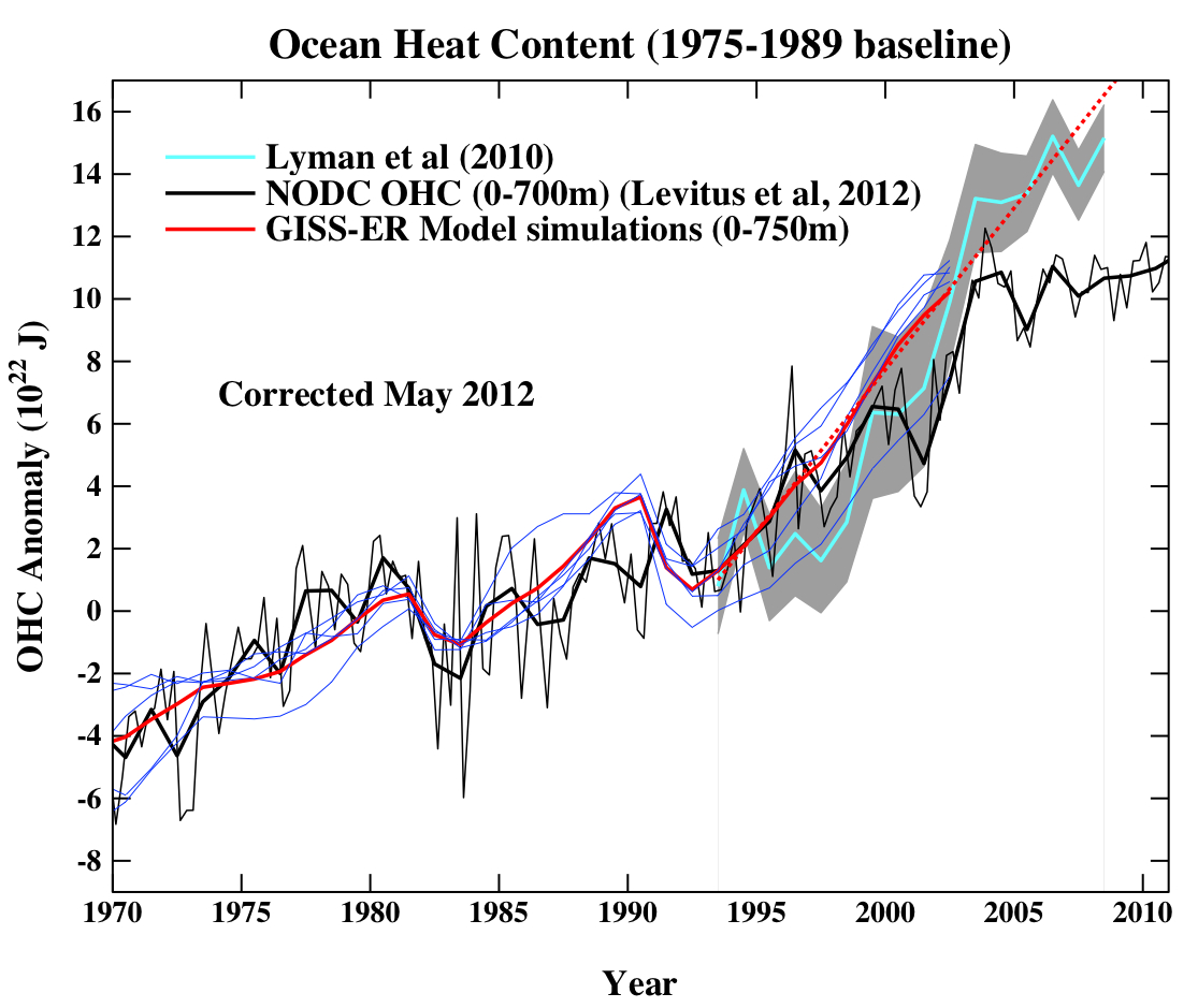 Original:
 Clearly the model extension in the chart reproduced by From Peru matches the original rather than the updated version.
-
Tom Curtis at 10:18 AM on 25 May 2012Modeled and Observed Ocean Heat Content - Is There a Discrepancy?
From Peru @9, with one important quibble, I agree with all that you say. However, the graph you showed shows a 0-2000 m GISS-ER predicted OHC that is well within error of the 0-2000 m OHC observed by Levitus et al. Consequently, I am unsure why you call it "ugly", nor why you think fake "skeptics" would like to use it. I suspect in the updated chart, the the predicted change in OHC will exceed the observed, but unfortunately do not have an updated graph to directly confirm it. That said, Dana extensively discusses this issue in the original post. He surveys a variety of observational estimates, most showing change in OHC of around 0.5 W/m^2, which compares to the 0.6 W/m^2 (GISS-EH)or 0.7 W/m^2 (GISS-ER). Given the differences in volume and time periods involved, it is difficult to assess if, and to what extent either model is in error, all though GISS-EH appears to do quite well. The important quibble is that, by changing the temperature of the Earth's surface, oceanic oscillations will change the radiative balance through changes in cloud cover and humidity (and other feedbacks). Specifically, if climate forcings have a positive feedback compatible with IPCC predicted climate sensitivities, decreasing global temperatures will result in a lower reduction in OLR than would otherwise be the case. In contrast, if feedbacks are negative, decreasing global temperatures will result in a larger reduction in OLR than can be accounted for by temperature differences alone. In the former case, a transition from El Nino to La Nina conditions will result in a reduction in the expected TOA energy imbalance. -
From Peru at 09:18 AM on 25 May 2012Modeled and Observed Ocean Heat Content - Is There a Discrepancy?
Tom Curtis: "The only real problem is that the model does not predict a hiatus period. As hiatus periods are associated with ENSO activity, this is not entirely surprising." The hiatus is a situation where the heat from radiative forcing is transferred to the deep ocean more efficiently, mainly because the ENSO system is dominated by the La Niña phase, with the consecuence that there is less heat in the upper ocean to warm it. It explains the slowdown of the upper 700 m increse in OHC (or at least part of it) and the flatness of sea surface temperature timeseries in the last decade. However, ENSO do not create or destroy heat (nor any other oceanic oscillation), just redistribute it. So, if the radiative forcing remains constant, and the upper ocean warms less, the deeper ocean must warm more. (By the way, Bob Tisdale might have discovered just this when he blames all global warming on the big El Niños (and their aftereffects) of the last 40 years. Too bad he do not consirered the law of conservation of energy when he claims that ENSO can warm the Earth without an external forcing) However, even going to 2000 m deep, the warming appear in some datasets to have slowed. This could be due to measurement errors, but is likely true because in the last decade there was a deep solar minimum and an increase in cooling aerosols emissions from Asia -
Tom Curtis at 08:46 AM on 25 May 2012Modeled and Observed Ocean Heat Content - Is There a Discrepancy?
dana@7, in FromPeru's chart, the final intersect between the extension of the 0-750 m predicted OHC and the 0-700 m observed from Levitus is in approximately 2007. In contrast, in the figure you show, the predicted 0-750 m OHC does not intersect the Levitus 0-700 m OHC after approx 1997. By visual inspection, there is no obvious difference in the baselining. That being the case, I am fairly certain FromPeru's chart is not an updated chart, even though it is listed as such in the RC post. Regardless, the chart shown on the RC post is the same chart as that shown if you follow the link to the "uncorrected" chart. So, either Gavin has accidentally displayed the uncorrected chart in the post, or accidentally linked to the corrected chart instead of the uncorrected chart. (Or I need to see an optometrist.) -
dana1981 at 08:34 AM on 25 May 2012Modeled and Observed Ocean Heat Content - Is There a Discrepancy?
Tom @5 - that graphic is updated. The previous version showed a better match between GISS-EH and Levitus data, but that was due to a mistake on Gavin's part, treating the model simulation as being in units of ocean rather than global surface area. There is a modest discrepancy between both 0-700 and 0-2000 (vs. full ocean) data and models there, but as I said, it's just one model (and in fact just an extrapolation of the mean of 5 simulations with that model), and just one OHC data set. Gavin's light blue line represents the ~0.7 W/m2 full ocean OHC GISS-EH mean model run, vs. the OHC observations generally being around 0.5-0.6 W/m2. -
dana1981 at 08:29 AM on 25 May 2012Modeled and Observed Ocean Heat Content - Is There a Discrepancy?
From Peru @4 - the answer is that particular graphic only shows GISS-ER vs. Levitus data. As noted in the post above, GISS-EH matches most OHC reconstructions better than GISS-ER, and Domingues (2008) shows several other models as well. -
Tom Curtis at 08:27 AM on 25 May 2012Modeled and Observed Ocean Heat Content - Is There a Discrepancy?
From Peru @4, that figure is drawn from the Real Climate post of Feb 8th, 2012. Unlike the other RC posts in which an OHC chart has been updated, the currently displayed chart does not note the update. Further, on visual inspection, I can find no difference between that chart and the chart you find if you follow the link to the uncorrected chart. This strongly suggests to me that the chart you show is not a corrected chart, but rather than Gavin has accidentally linked to the old chart when making his update. In any case, the chart you show shows essentially no discrepancy between model and data for 0-2000 m, and good correlation for 0-700 (750) m. The only real problem is that the model does not predict a hiatus period. As hiatus periods are associated with ENSO activity, this is not entirely surprising. -
empirical_bayes at 08:18 AM on 25 May 2012Hansen and Sato Estimate Climate Sensitivity from Earth's History
@HumanityRules, #6 03:13 AM on 24 May, 2012: It is hard to to see how the Schmittner curves mix. (snip)Moderator Response: TC: Of topic text snipped. I would greatly enjoy further exploration of the snipped text in a thread where it is on topic. Unfotunately it is off topic here, and consistency requires that I moderate based on compliance with the comments policy, not personal agreement or disagreement with points being made. -
From Peru at 07:45 AM on 25 May 2012Modeled and Observed Ocean Heat Content - Is There a Discrepancy?
There is a corrected graph that is very ugly: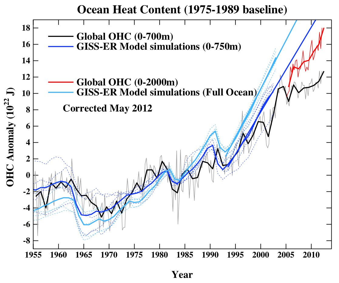 The "skeptics" will surely use it everytime they can.
What answer can be given to them (and specially to the true skeptics that are victims of the disinformation that the fake skeptics spread everywhere)?
There are any models that, unlike the ones shown in the figure, follow reality?
The "skeptics" will surely use it everytime they can.
What answer can be given to them (and specially to the true skeptics that are victims of the disinformation that the fake skeptics spread everywhere)?
There are any models that, unlike the ones shown in the figure, follow reality?
-
dana1981 at 07:24 AM on 25 May 2012Modeled and Observed Ocean Heat Content - Is There a Discrepancy?
Albatross @2 - I certainly agree that relying on one's eyecrometer is rarely a good idea. Particularly when comparing data across different timeframes or different parameters (i.e. 0-700m vs. 0-2000m) - in that case the eyecrometer is essentially useless. That's why I wanted to try and do the analysis properly, to see if the numbers show there really is a discrepancy. As the post notes, it's hard to say, but it's possible (the uncertainties are just too large to say for sure either way). Certainly nowhere near a factor of 2 discrepancy though. -
Albatross at 06:58 AM on 25 May 2012Modeled and Observed Ocean Heat Content - Is There a Discrepancy?
Dana, In addition to the disinformation that "skeptics" are spreading on this issue, Roger Pielke Senior continues to try and undermine Levitus et al. (2012) (and James Hansen's research) by making unsubstantiated and subjective assertions/challenges. Pielke Senior claims that "This is a discrepancy of ~2 between his prediction and the analysis of Levitus et al 2012 if the latter observational analysis is correct." This is incorrect. One has to compare the data for the same time windows and for the same depth range. Comparing a rate for 1955-2010, with one for 1993-2003 as Pielke does is ludicrous. Pielke Senior then goes on to try and defend his (incorrect) conclusion by claiming that "While one possibility is that the rate increased after 1993 compared to earlier in the 1955-2010 period, but visually (using the eyecrometer) this does not seem to be the case." I do not know why Pielke chooses to rely on the notoriosly innacurate and subjective "eyecrometer" method when one can download the Levitus et al. (2012) data and calculate some statistics. Additionally, Pielke is applying his eyecrometer to the 0-2000m data here (the image from Levitus et al in his post) while actually making reference to the 0-700 m data. So instead of using the "Pielke eyecrometer™" let us look at the 0-700 m data for Levitus et al. shall we? The slope for 1955-2011 for 0-700 m is 0.26x10^22 J/yr, while for 1993-2011 the slope is 0.58x10^22 J/yr. So the slope from 1993 to present is more than double that for 1955-2011. Pielke Senior also alleges that "Levitus et al 2012 may be overstating the magnitude of recent upper ocean heating as clearly seen in the figure below from NOAA’s Pacific Marine Environmental Laboratory" This is simply not true. Analyzing the Pacific Marine Environmental Laboratory (PMEL) data (available here) we get a rate/slope of 0.78x10^22 J/yr between 1993 and 2011, which is greater than the rate (0.58x10^22 J/yr) obtained using the Levitus et al. data for the same depth range and the same period. So reality is again the complete opposite to Pielke's assertion and his "Pielke eyecrometer™" is telling him. Pielke Senior is engaging in very bad scientifc practice when he makes grandiose (and as it happens incorrect)proclamations based on nothing more than subjectively eyeballing graphs. -
zinfan94 at 05:44 AM on 25 May 2012Hockey stick is broken
There is a recent paper by Gergis et. al., discussed yesterday in a post on RealClimate site, that covers proxies for Australia and Oceania and results in a hockey stick. it would be interesting to see this SH Australasia hockey stick from Gergis(2012) compared to the Mann(2008) hockey stick, on the same timescale, displayed one above the other. I used the Gergis image from RealClimate, and the Mann image from the SkS site, and there seems to be some interesting agreement periods. For example, the sharp drops in proxy temperatures around 1350 and 1460 are present in both records, as near as I could see. From what I understand, sometimes the NH and SH temperatures will march together, and other times be out of phase. Perhaps SkS could discuss the two proxy records, comparing the temperature swings, written by someone knowledgeable of likely temperature swings over the last 1200 years. -
dana1981 at 02:50 AM on 25 May 2012Modeled and Observed Ocean Heat Content - Is There a Discrepancy?
Also kudos to Gavin Schmidt for so quickly noting and correcting the mistake in his prior model-data comparison posts. That's how true skeptics behave. -
Martin A at 23:59 PM on 24 May 2012CO2 has a short residence time
Dikran M: Thank you - I'll go back and look more carefully at your paper. I had thought the examples I had worked out (including the one above) had shown that residence and adjustment times were the same for a 1st order linear system. I think you are quite right. It makes good sense to reconcile your model and mine before introducing any further complications. -
dana1981 at 15:17 PM on 24 May 2012Hansen and Sato Estimate Climate Sensitivity from Earth's History
Fair point Tom, they certainly consider various LGM temperature reconstructions which use both terrestrial and ocean data. -
Tom Curtis at 14:23 PM on 24 May 2012Hansen and Sato Estimate Climate Sensitivity from Earth's History
dana, thank you for clarifying about the qualitative nature of the ESS. With regard to your discussion with HR, I believe he has overstated his case, but is correct that H&S use terrestrial data in determining the climate sensitivity. H&S use the ocean core data to establish relative temperature over the last 800,000 years, and show that, with their estimated forcings and a fast feedback sensitivity of 3 degrees C per 4 W/m^2 of forcing, predicted and observed temperatures correlate near perfectly. However, as they note, an equally good correlation would be achieved if temperatures and sensitivity were each scaled by the same factor. Therefore, different assumptions about global temperatures at the LGM result in different, and consistent estimates of the fast feedback sensitivity. As they say:"Global temperature change calculated by multiplying the sum of the two climate forcings in Fig. 5c by climate sensitivity ¾°C per W/m^2 yields a remarkably good fit to the "observed" temperature (Fig. 6). The observed temperature is based on the assumption that 4.5°C is a reasonable approximation of the LGM-Holocene surface temperature change, and thus a scale factor of 2 is used to convert δ 18 O deep ocean temperature change (equation 6) to surface temperature change. However, we could obtain an equally good match between the temperature calculated from the forcings and the temperature from δ 18 O if we assumed the LGM-Holocene warming was 6°C and fast-feedback climate sensitivity was 1°C per W/m^2 , or if we assumed that the LGM-Holocene warming was 3°C and climate sensitivity was 0.5°C per W/m^2. If LGM cooling is so uncertain as to be anywhere in the range 3-6°C, we can only conclude that the fast-feedback climate sensitivity is 3 ± 1°C for a 4 W/m^2 CO2 forcing. Thus accurate knowledge of the global temperature change between glacial and interglacial states is needed for empirical evaluation of fast-feedback climate sensitivity."
In order to constrain the temperatures at the LGM, Hansen and Sato discuss a variety of estimates, noting the inconsistency of sst based estimates such as CLIMAP and MARGO and terrestrial proxies. Finally, they state:"Given the inconsistencies among proxy data sets, our present assessment of global LGM cooling must be partly subjective. Our central estimate, 4.5°C, chosen with cognizance of discussions in the past three decades as new data sets were compared with CLIMAP, is in the middle of the range in the paleoclimate literature. Given that a global atmospheric model driven by CLIMAP sea surface temperatures yields LGM cooling of 3.6°C (Hansen et al., 1984), and indications that CLIMAP sea surface temperatures are incompatible with terrestrial data as well as with some marine data, we believe it is unlikely that global LGM cooling was much less than 4°C. On the high side, we argue that it is unlikely that global LGM cooling was much more than 5°C, because (1) LGM Antarctic cooling averaged over the Vostok (Vimeux et al., 2002) and Dome C (Jouzel et al., 2007) sites was 8-9°C, while both climate models and empirical data typically yield polar amplifications of quasi-equilibrium temperature change close to a factor of two, (2) despite disagreements about LGM ocean temperatures, there is general agreement that LGM cooling was limited in the tropics and subtropics."
Thus they explicitly adopt an estimate greater than those based on CLIMAP and MARGO, and explicitly do so because of the inconsistencies with terrestrial data. However, they do not simply adopt an estimate based on terrestrial data, which would lead to a temperature estimate for the LGM closer to 6 degrees C below the pre-industrial average. -
HumanityRules at 13:23 PM on 24 May 2012Hansen and Sato Estimate Climate Sensitivity from Earth's History
From section 5 "Our estimate of LGM global cooling is thus 4.5±0.5°C," "Our estimated LGM-Holocene forcings with 1σ uncertainties are 3±0.3 W/m2 for GHGs" I'd agree they are deriving these figures from a 'review' of other work but they seem to be presenting there own opinion as well. The second quote you use is from this section also. It actually seems like a strange add-on to the paper, I'm not sure of the purpose of it. -
dana1981 at 13:11 PM on 24 May 2012Hansen and Sato Estimate Climate Sensitivity from Earth's History
HR @10 - yes, HS12 only uses ocean core data for their temperature reconstruction. In the section you quote they're only talking about other studies. -
HumanityRules at 13:08 PM on 24 May 2012Hansen and Sato Estimate Climate Sensitivity from Earth's History
(Section 5 of Hansen's paper) -
dana1981 at 13:06 PM on 24 May 2012Hansen and Sato Estimate Climate Sensitivity from Earth's History
Tom @9 - the first section is just an introduction, and Figure 1 is labeled as a schematic in the caption. However, I have added a note about the greater uncertainty regarding long-term sensitivity in the ESS section in the post. -
HumanityRules at 13:02 PM on 24 May 2012Hansen and Sato Estimate Climate Sensitivity from Earth's History
Dana says "HR @6 - Hansen's temperature estimates in this case are based on deep ocean δ18O." Are you sure? We are both talking about the LGM section of the paper? We're Hansen talks about "the less ambiguous terrestrial data" and where he criticizes Schmittners use of MARGO (oceanic) data? The deep ocean stuff seems to relate to the Cenozoic part of the paper. -
amhartley at 10:36 AM on 24 May 2012If you want them to remember, tell a story
How could I fail to mention the parables of Jesus? "I will open my mouth in parables, I will utter what has been hidden since the foundation of the world." (Matt. 13:35) Not all parables were stories, but most were. -
Muzz at 09:20 AM on 24 May 2012If you want them to remember, tell a story
Exactly the technique used by Australia's own Climate Commissioner. He's brilliant at it. -
Bob Lacatena at 09:17 AM on 24 May 2012New research from last week 20/2012
From Peru, I'm not sure why you don't see the data you want at the NOAA site. For instance, look at this page and click "Get Yearly Data" near the bottom. -
Tom Curtis at 09:13 AM on 24 May 2012Hansen and Sato Estimate Climate Sensitivity from Earth's History
Dana, I believe your first section is insufficiently clear. H&S 2012 refine their previous estimates of the fast feedback climate sensitivity using empirical data over the last 800,000 years. However, there representation of slow feedback climate sensitivity is characterized as a "schematic", and is not an empirical result. They highlight certain empirical events such as the PETM, and from features of those events, deduce qualitative features of the Slow Feedback Climate Sensitivity - but that does not make that figure an empirical conclusion. As an example, the entire justification peculiar peak in the center of the Fast Feedbacks plus Albedo curve (just to the right of holocene conditions is:"Also, in sketching the Earth system climate sensitivity we bear in mind the possibility of a hysteresis effect that makes demise of the Antarctic ice sheet difficult, thus stretching out toward larger forcing the ice sheet addition to the fast-feedback sensitivity."
Hysteresis with respect to the Antarctic Ice sheet is probably a significant factor in Earth System Sensitivity, but it may modify the curve by first depressing it than elevating it, ie, by introducing a sine wave pattern rather than a simple peak. The reasoning does not even justify the shape of the curve, let alone the magnitude of the effects. I do not fault Hansen and Sato on this, as they are quite clear that their figure 7 (your figure 1) is a "schematic". I think that important qualification is eroded, however, when you describe the graph as their "climate sensitivity conclusions". -
funglestrumpet at 08:51 AM on 24 May 2012If you want them to remember, tell a story
Vroomie @ 1: From cars to karst - was it a bumpy ride? You may have hit on why Monckton is so popular. He in effect tells a story along the lines of a fairytale that climate change is no problem. And like Bill Harly, he puts on a show while telling it. -
From Peru at 07:57 AM on 24 May 2012New research from last week 20/2012
Sphaerica: Thank you for the link, (where I found the PDF of the paper) but ... ...I still don't find from where do Levitus et al. obtained the pre-2005, 2000-meter deep Ocean Heat Content and Thermo-Steric Sea Level Rise (in the paper, Figure 1 show the World Ocean Heat Content for the 2000m deep layer since 1955).
Prev 1160 1161 1162 1163 1164 1165 1166 1167 1168 1169 1170 1171 1172 1173 1174 1175 Next


