Climate Science Glossary

Term Lookup

Enter a term in the search box to find its definition.

Settings

Use the controls in the far right panel to increase or decrease the number of terms automatically displayed (or to completely turn that feature off).

Term Lookup

Settings


All IPCC definitions taken from Climate Change 2007: The Physical Science Basis. Working Group I Contribution to the Fourth Assessment Report of the Intergovernmental Panel on Climate Change, Annex I, Glossary, pp. 941-954. Cambridge University Press.

Home Arguments Software Resources Comments The Consensus Project Translations About Support

Twitter Facebook YouTube Mastodon MeWe

RSS Posts RSS Comments Email Subscribe


Climate's changed before
It's the sun
It's not bad
There is no consensus
It's cooling
Models are unreliable
Temp record is unreliable
Animals and plants can adapt
It hasn't warmed since 1998
Antarctica is gaining ice
View All Arguments...


Username
Password
New? Register here
Forgot your password?

Latest Posts

Archives

Graphs from the Zombie Wars

Posted on 6 January 2011 by keithpickering

Cross-posted at The Numerate Historian

There are a few of us who actually enjoy arguing with “climate zombies” (a term coined by Joe Romm at ClimateProgress, and one too often apt) in comments and political forums online. If you hang around long enough, you’re bound to hear some of the silliest crackpottery one can imagine. For a long time Skeptical Science has been an important resource for me, so I’m happy to have a chance to give back.

Recently, I pointed out to an adversary that CO2 and temperature were highly correlated, and to support my assertion I posted the following graph, which I did in Excel. For these graphs, the temperature data is from HADCRUTv3; and the CO2 data is from two sources: Mauna Loa (1959-2009) and the Law Dome ice core (pre-1959; using the 20-year smoothed values).

tempCO2

The blue CO2 line overlays the red Temperature line very nicely, and shows the relationship quite well. But there’s a big problem here: there is no vertical scale. And in fact, there can’t be a single vertical scale on a graph like this, because the two lines are valued very differently: temperature anomaly, in degrees Celsius, ranges between –.8 and +.6, while CO2, in parts per million, ranges between 280 and 390. In order to get the two lines to overlay in Excel, I had to alter the scale of the temperature line quite significantly, by multiplying each datapoint by a constant and adding a second constant. Ideally, I would like to put two vertical scales in place so that each line could be scaled separately. But Excel won’t allow that. Of course, adding and multiplying by constants makes no difference at all to the correlation; but my opponent was unimpressed and immediately accused me of data manipulation. How do you counter an argument like that when your opponent is nearly innumerate?

One thing you could do is draw two vertical scales on the graph, to make things perfectly explicit. Excel won’t do that, but there is other software out there that does. I happen to be familiar with GMT, an open-source mapping tool that also has extensive graphing capabilities. So let’s re-create the above graph in GMT but with two vertical scales, one for each dataset. Here is the result:

CO2

Well that’s better, but some zombies just won’t die. My opponent decided to attack the whole idea of correlation because, he claimed, the data wasn’t linear and therefore drawing a correlation coefficient wasn’t valid. The argument is utterly bogus, of course, but sometimes you can find interesting jewels even when rebutting the obviously silly. Here’s what I came up with: we eliminate the date from the graph and just plot CO2 against the global temperature anomaly in a scatterplot.

HAD-co2

Now the strong linear relationship jumps out at you as big as life and impossible to miss. I like this graph so much that the next time someone tries to tell me that CO2 and temperature aren’t correlated, or that there's no proof that CO2 causes higher temperatures, this is the first graph I’m going to use. For the entire 160-year period, the Pearson correlation coefficient r = .89, which is highly significant.

And before anyone reading this jumps on me – yes, I realize that the relationship here is based on radiative forcing, and therefore should theoretically be logarithmic and not linear. But first, the range of CO2 values is too small here to show much of a curve; and second, forcing isn’t the only factor at work: there is also feedback to consider, which might drive the actual relationship toward linear or even worse, if for example long-term feedbacks are more positive than short term feedbacks (as seems likely). So the graphed linear relationship isn’t necessarily wrong, and certainly seems empirically justified for this range of values.

One interesting thing you can do with a graph like this is to (very roughly) estimate climate sensitivity to CO2 forcing, by finding the equation of the regression line (shown in black). The equation of that line in the graph above is: T = .0085C - 2.83. From this we can determine that the mean temperature anomaly for the pre-industrial CO2 value of 280 ppm would be ?.46, and for the doubled CO2 value of 560 ppm it would be expected to come in at +1.92; therefore doubling CO2 should raise the Earth’s temperature by about 2.38° C. This is in the ballpark of many recent (and much more sophisticated) estimates – though perhaps a bit on the low side; most recent estimates are in the range of 2° to 4.5° C increase for doubling of CO2, though some are as high as 6° C.

But then again, we’re using HADCRUT data, which omits much of the rapidly-warming polar regions of the Earth. We can switch to NASA’s GISS dataset, which loses 30 years of early data but which includes the poles, and draw a similar scatterplot.

GISS-co2

Here the correlation coefficient is unchanged at r = .89, but the regression slope is a little higher. For these data, T = .0096C - 3.05, and following the same procedure as above the regression line implies that doubling CO2 should raise global temperature by 2.68° C – which is still in the ballpark (but perhaps still a bit low). Still, not bad for a back-of-the-envelope calculation using publicly available data.

0 0

Printable Version  |  Link to this page

Comments

Prev  1  2  

Comments 51 to 80 out of 80:

  1. That CO2 and temperature appear highly correlated is a coincidence although there is an underlying explanation. There is no need for CO2 and temperature to be correlated for there to be cause and effect. Emphasising a coincidence at the expense of cause and effect is a mistake and does not clarify AGW arguments. Consider what would happen if a large pulse of CO2 had been added to the atmosphere. The effect would be one of increasing temperatures, rising quickly at first and then more slowly to a new stable value. The CO2 concentration would be constant with time however. ie there would be no correlation but there would be cause and effect. What would happen if CO2 then fell? There would be rising temperatures while CO2 was falling and eventually falling temperatures when CO2 was constant again. The correlation you see is in fact a coincidence due to the historical pattern of anthropogenic and natural forcing. That is temperature and CO2 concentration have changed in a similar way but for different reasons. This point does of course mean that those who see the apparent correlation and assume temperature must be driving CO2 are equally misguided. That the coincidence happens is because a steadily increasing forcing results in an accelerating temperature rise. CO2 additions to the atmosphere have increased exponentially but this can be well approximated by a 2nd order polynomial, as can the temperature rise. Since these are similar curves they appear correlated. That they can appear similar at all is because all the long term forcings are changing slowly and smoothly. When forcing changes abruptly correlation is lost. Had our CO2 emissions been more erratic we could still have seen a similar temperature curve and have the same total CO2 emitted but there would be poor correlation between CO2 levels and temperature. To demonstrate that the temperature rise is related to the CO2 change requires a more sophisticated analysis accounting for the many different variables and consideration of some simple physics. This correlation is coincidental. It is neither necessary nor sufficient as the basis of an argument in support of CO2 induced warming. Conversely a lack of correlation does not disprove CO2 induced warming either.
    0 0
  2. Interesting, in that you "prove" that the correlation is coincidental, only by using an example that assumes that is it causal in the first place. Perhaps you would like to try again? Also, when you say that the temperature changed for a different reason than CO2 forcing, what other forcing are you assuming has caused the current warmth? Because pretty much every other idea out there has already been falsified. Finally, while it's true that correlation does not prove causation, in this case the causal mechanism is well known basic physical chemistry. Can we assume that the laws of science have not been suspended, and therefore that CO2 does indeed make the planet warmer?
    0 0
  3. You have to plot the forcing 5.35 Ln (C/Co) where C is the CO2 concentration in ppm to get anything sensible. The favorite trick of the denial ducks is to squeeze one axis or the other.
    0 0
  4. 40 million years ago, when the Sun was a bit dimmer than it is now and the latitudinal distribution of the continents was almost exactly the same as it is now (i.e. same land-albedo forcing as present), the Earth was too warm to cycle in and out of glacial periods. In fact, the Earth's poles were essentially ice-free at that time. For those who think that the CO2-lags-temperature argument is a valid argument against global-warming theory, here's a question: Why was the Earth so warm then? (Now remember that solar + land-albedo forcing was the same or a bit less then than it is now).
    0 0
  5. That's a point I often make, caerbannog. From my reading, the planet was around 6 degrees warmer, then, than during the bulk of the Quaternary Era-in spite of a much dimmer sun. Of course, CO2 levels in the atmosphere were anywhere from 3 to 10 times higher than the Quaternary too!
    0 0
  6. #51: "Since these are similar curves they appear correlated. That they can appear similar at all is because all the long term forcings are changing slowly and smoothly." The curves are similar because there is a genuine physical cause for their similarity: increasing CO2 concentration increases CO2 forcing in a predictable way. Your argument is based on the (deliberate?) omission of this obvious fact -- and that is why it must be so tortuously circular. See CO2 effect is weak and any of the many threads on climate sensitivity to forcing. See the graph here for the relative strength of the long-term forcings; there can be no doubt that CO2 is the key.
    0 0
  7. can you show an additional plot related to your figure three to show monthly co2/temps? i have done this and i see a flattening of the curve at co2 of around 375 ppm and the temps are flat above that region. your yearly graph seems to show the same thing. if i had a web site i'd post the graph and don't know how to show it along with the data in this comment field. i took the hadcrut3 monthly global temperature anomalies on the y-axis and the mauna loa monthly co2 ppm on the x-axis. there was a very pronounced 'flattening' of the curve past 375 ppm. why is that?
    0 0
  8. well, that didn't work either. i'm sorry about cluttering your site up. please delete the other posts too. ugh!
    0 0
    Moderator Response: [Daniel Bailey] You are almost there. Try linking to a PNG or other graphics file instead of a PDF (PDF's will not link as a visual graphic in a SkS comment window).
  9. While I disagree with your conclusions you did a magnificent job with this post.
    0 0
  10. @garythompson: I think I see what you're looking at, but it's an optical illusion. Two ways to check: first, plot the graph with axes switched, like this: co2TempMonthly 
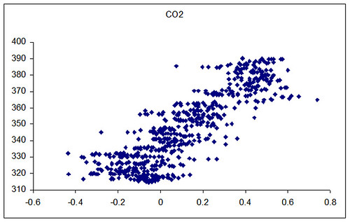
... and any "flatness" should become verticality, which is not evident to my eye. More formally, check to see if the linear regression fit is improved by a polynomial fit. In this case, it isn't much improved ... but more importantly, the best 2-order polynomial fit is actually concave upward, i.e., the curve is accelerating rather than decelerating.
    0 0
  11. A few days ago I came across a paper provocatively titled “Unskilled and Unaware of It: How Difficulties in Recognizing One’s Own Incompetence Lead to Inflated Self-Assessments" (PDF available here). It received an Ig Noble Prize in 2000 and is definitely worth a look. Some of those doing battle with the Zombies may find it insightful.
    0 0
  12. I see that some of the zombie responses that I highlighted above, have re-appeared on another thread ( Understanding the CO2 lag in past climate change), courtesy of a poster called apiratelooksat50 : "...it is far more prudent and cost-effective to adopt a wait-and-see approach than to spend trillions now on what may or may not be a problem." "...it would be necessary to shut down the entire global economy for a decade." "By adopting a wait-and-see approach, we still have plenty of time to address even the worst-case predictions of climate change." Pure zombie-opinion in place of facts or evidence, as usual. But there were a couple of extra zombie arguments also, that I forgot to mention : "Or, we could feed and educate everyone in the world." "Even if global warming becomes a problem, it’s going to be a problem regardless of how much we spend." "Initially I was pro-AGW, but over the years as I've witnessed the shouting down and negative labeling of legitimate scientific inquiry that questioned components of the AGW theory, my position changed. Real science is always open to refutation and revision." You often see the supposed 'concern' for the poor and starving of this world (alongside the false supposition that all problems could be solved, and that the poor and starving wouldn't continue to suffer, if only we spent all that money - money which shouldn't really be spent anyway, as far as the zombies are concerned - on food and education); as well as the shoulder-shrugging, 'so what, we can't do anything about it anyway (even if it is a problem), so why should we bother' attitude; and the 'I used to be convinced about AGW but seeing the horrid attitude to the brave deniers (as I now realise they are), I was convinced otherwise and have disregarded the science in favour of standing with the oppressed and ever-courteous Galileo-like real skeptics like, um, Watts and, er, McIntyre', and some others. Laughable, but bizarre.
    0 0
  13. @60 Keith: if my accelerating you mean more CO2 means temperatures going faster, there's no good physical reason for that yet afaik. It's probably because this only looks at CO2 forcing and not total forcing. Aerosol's negative forcing hasn't grown as quickly as CO2's has. Assuming that it is negative and not increasingly negative at the same rate that CO2 is increasingly positive, then it would give the illusion of more impact from CO2 and acceleration.
    0 0
  14. Muoncounter #48 Nice job. Humbled that a distinguished contributor such as yourself is naming a law after me. Not bad for a 'zombie'. Of course you are considering only one component of the forcing ie CO2GHG via the log function. I have not found any equations for the WV + Ice Albedo feedback climate response or cloud cooling forcings - and we know that S-B cooling is proportional to T^4. However assuming that you CO2 component only curves are worth talking about, the temperature anomaly is tracking somewhere between 1.2 and 1.8degC for a doubling of CO2. Oft quoted and AGW consensus number is more like 3.0degC for a doubling of CO2 from pre-industrial levels. Since we have already had 0.75-0.8 degC warming since AD1750, this suggests we have 0.4 - 1.0 degC to go at doubling. Not so scary after all.
    0 0
  15. #63 MarkR: You're right, no physical reason, and the polynomial fit isn't enough better than linear to be worth talking about at all -- except that it shows that the apparent flatness is illusory. #64 Ken Lambert: "However assuming that you CO2 component only curves are worth talking about, the temperature anomaly is tracking somewhere between 1.2 and 1.8degC for a doubling of CO2." That number is derived from radiative physics only, so it excludes all feedbacks. The rough estimate from linear regression above includes short-term feedbacks (at least), e.g., water vapor. Which accounts for the difference.
    0 0
  16. #54 @caerbannog For those who think that the CO2-lags-temperature argument is a valid argument against global-warming theory, here's a question: Why was the Earth so warm then? (Now remember that solar + land-albedo forcing was the same or a bit less then than it is now). Well, it comes that CO2 concentration was much higher then than now. http://www.sciencemag.org/content/330/6005/819.abstract This as been discussed here before: http://www.skepticalscience.com/Climate-change-from-40-million-years-ago-shows-climate-sensitivity-to-CO2.html
    0 0
  17. Ken Lambert, between 1750 & 1950, there was only a 20ppm increase in CO2 concentrations. Since 1950, there has been an 80ppm increase in CO2 concentrations. So really, the important part is how much temperatures have risen since 1950, not 1750 (when the CO2 effect was being masked by the negative forcing of aerosols). Since 1950, we've seen a +0.6 degree increase in *global* temperatures-so what impact do you reckon *another* 80ppm rise in CO2 will do over the next 60 years alone? Of course, that's *before* we consider the reduced albedo effects from melting ice & glaciers-which is a positive feedback-or the impact of clouds, or the impacts of methane release from clathrates. Also remember that this represents an *average* warming only-some parts of the world will warm much more than others-enough to make them effectively uninhabitable. Are you going to tell refugees from these parts of the world (Asia, the Middle East & Sub-Saharan Africa come to mind) that a "mere" 0.8 degree warming is "nothing to be scared of"? Still, got to give kudos for squeezing so many Zombie memes into a single post.
    0 0
  18. A couple of weeks ago (when some uncharacteristically rainy weather kept me indoors here in San Diego), I decided to "roll up my sleeves" and write up my own simple global temperature-anomaly program. Nothing fancy -- all it does is compute NASA-style annual temperature anomalies for all of the GHCN stations and then perform simple "dumb averages" to come up with crude global annual temperature anomaly estimates. No fancy gridding/geospatial weighting or anything like that -- just simple plain-vanilla dumb averages of the anomalies. I crunched both the GHCN *raw* and *adjusted* monthly-mean temperature data sets. Since most of the GHCN temperature stations are located in the temperate regions of the NH, I snagged NASA's "Northern Latitudes" temperature anomaly data from the GISSTEMP repository to see how my own results compared with some official NASA results. Below is a plot of the results (5-year moving averages): My "dumb average" GHCN raw data results are plotted in green. My "dumb average" GHCN "adjusted" data results are plotted in red. And NASA's official "Northern Latitudes" temperature anomalies are plotted in blue. The results pretty much speak for themselves. This was not a difficult task at all. I'm an EE with so-so programming skills (my technical abilities would best be measured in either MicroSanters or MegaWatts), and this was a slam-dunk easy programming exercise. This is exactly the sort of project (broken up into digestible chunks) that would be good to assign bright college-bound high-school students (calibrated to USA academic standards here). Now the question is -- why didn't any of the loud-mouthed Wattsian deniers who have been accusing NASA/CRU/etc. of "cooking the books" with temperature "adjustments" perform some simple sanity checks like this on the data *years* ago? I mean, if you are going to proclaim loudly and publicly that NASA's global-warming results are artifacts of "temperature adjustments", wouldn't you want to verify that by crunching the raw vs. adjusted data yourself before shooting off your mouth? (rhetorical question here).
    0 0
  19. Caebrannog @68, Don't sell yourself short! I also found your interpretation of the numbers very interesting. Readers can find his/her summary here at Tamino's place.
    0 0
  20. caerbannog @ 68 - Nice job. Fancy writing a rebuttal?.
    0 0
  21. Dear Keithpickering I am very pleased with your opening statement of this blog post. I have been able to verify the graphs from the links you have given. The following remarks should be seen as a supplement and I would suggest that you make this analysis and add it to the blog post: If you have two independent time series with a linear trend, you will find graphs like those shown by keithpickering. If you calculate the year to year differences in temperatures and in CO2 concentrations and plot them, then you will find no correlation. This is no coincidence, but can be proven mathematically for all such series as well as by simulations. The trick of taking year to year differences is used to prove that there is no correlation between temperature and CO2 concentration is used by Paulo Cesar Soares in his publication: http://www.scirp.org/Journal/Home.aspx?IssueID=465#3447 Please refer to Figures 11 /12 on pages 107/108. It will be interesting to read the reactions from the skeptical blogs and from the peer reviewer’s when they have understood the methods used by Paulo Cesar Soares to prove that there is no correlation.
    0 0
  22. #71: "If you calculate the year to year differences in temperatures and in CO2 concentrations ..." A very similar approach was taken by G.T. Wilson here, with apparently very good correlation. The most significant and best estimated effect is the dependence of temperature on the rate of increase of CO2, i.e. the change in the current value of CO2 from its value the previous year. This accounts for much of the variation of temperature about its trend. It also accounts partly for the trend in temperature, because the rate of increase of CO2 is itself increasing over the period. He also found a strong correlation between atmospheric CO2 and oil prices: Although the long term pattern of oil prices is positively correlated with (trend corrected) CO2, the spectral analysis correctly identifies the negative effect of the price increases, without which economic activity and CO2 emissions would have been even greater. What better means of establishing not just a contribution, but the anthropogenic control over atmospheric CO2?
    0 0
  23. Mucounter @72, Thanks-- interesting work by Wilson. A recent paper by Kodra et al. (published in a peer-reviewed journal) demonstrates that the radiative forcing from CO2 Granger causes global SAT. They also examine the role of ENSO. They conclude that: “The results from this modified test show evidence for Granger causality from a proxy of total radiative forcing (RC), which in this case is a transformation of atmospheric CO2, to GT [globally averaged land surface temperature]. Prior literature failed to extract these results via the standard Granger causality test. A forecasting test shows that a holdout set of GT can be better predicted with the addition of lagged RC as a predictor, lending further credibility to the Granger test results.” I would not place much weight on the Soares paper given that it appears in the same journal which just published yet another sub-par paper by Douglass. In fact, it is not even clear whether or not the paper was peer-reviewed. Is the "International Journal of Geosciences" becoming the new E&E for contrarians? Perhaps someone (e.g., DeepClimate) should do some digging around and about the journal's history..... PS: The link was working a while ago, but a quick test before posting now indicated that the Springerlink site may be down.
    0 0
  24. #73: "the new E&E for contrarians" There was a link in another thread to the same journal a couple of weeks ago. They still haven't published anything in their much-anticipated Advances in the Internet of Things. Here's a link to a presentation by Kodra on Granger. Rapidly approaching my limit on statistical analysis.
    0 0
  25. @Klaus: that journal you're linking to doesn't seem very credible. This is the title of one of the articles they posted: "“Molecular genetic program (genome) contrasted against non-molecular invisible biosoftware in the light of the Quran and the Bible” You can read more on the nebulous SCIRP in a Nature exposé.
    0 0
  26. @Klaus Flemløse Soares failed to find a correlation in monthly values, a totally unsurprising result. The lag between forcing and temperature change will always be longer than that.
    0 0
  27. Klaus Flemløse - Soares works with extremely short (months and 6-month periods) to examine his correlations; as keithpickering pointed out this is far too short. In looking at longer term correlations, he fails to account for other forcings (such as mid-century aerosols, which counteracted a great deal of CO2 forcing), which is quite a serious mistake. It's a very poor paper. This journal is very curious, both in article content and the mysteries of who is putting it out - previous comments have noted this as well. I would be very careful about accepting the articles based on it's (very short) history.
    0 0
  28. #64 keithpickering Well we have the log equation for forcing F.CO2, but do we have equations for all the other terms (cloud albedo etc) and the climate response feedbacks? eg. We know S-B if we know the effective radiating temp which is then dependent on the temp difference across the atmospheric column which is dependent on the WV + ice feedback etc etc etc. If we take the forcings from Dr Trenberth's Fig 4 (August09 paper) the net warming imbalance is 0.9W/sq.m. The net is what is important here - not any one forcing. If these forward temperature projections are worth anything, the forward forcings must be knowable to a reasonable degree of accuracy.
    0 0
  29. Co2 and Global temperatures Muoncounter @ 72 Tanks for the link to T.G. Wilson Albatros @ 73 Thanks for the link to Kodre et al – it will take some time to digest this paper Archiesteel @ 75 I was surprise about Soares conclusion from Figures 10/11. Then I found out that taking year to year differences in two independent time series always will produce zero correlation. That my point of view. This can be proven mathematically or by simulation. This will also be true for the time series Keithpickering has used. Given me time and I will produce the graphics. The Soares conclusions in respect of these graphs are either caused by lack of knowledge or bad will. This result will be repeated again and again on skeptical blogs.Be prepared!
    0 0
  30. Keith Pickering, Even Lubos Motl likes your post even though he has a quibble with the arithmetic. http://motls.blogspot.com/2011/01/climate-sensitivity-from-linear-fit.html Any comment?
    0 0

Prev  1  2  

You need to be logged in to post a comment. Login via the left margin or if you're new, register here.


The Consensus Project Website

THE ESCALATOR

(free to republish)


© Copyright 2024 John Cook
Home | Translations | About Us | Privacy | Contact Us