


 Arguments


A Frank Discussion About the Propagation of Measurement Uncertainty
Posted on 7 August 2023 by Bob Loblaw, jg
Let’s face it. The claim of uncertainty is a common argument against taking action on any prediction of future harm. “How do you know, for sure?”. “That might not happen.” “It’s possible that it will be harmless”, etc. It takes on many forms, and it can be hard to argue against. Usually, it takes a lot more time, space, and effort to debunk the claims than it takes to make them in the first place.
It even has a technical term: FUD.
Acronym of Fear, uncertainty, and doubt, a marketing strategy involving the spread of worrisome information or rumors about a product.
During the times when the tobacco industry was discounting the risks of smoking and cancer, the phrase “doubt is our product” was purportedly part of their strategy. And within the climate change discussions, certain individuals have literally made careers out of waving “the uncertainty monster”. It has been used to argue that models are unreliable. It has been used to argue that measurements of global temperature, sea ice, etc. are unreliable. As long as you can spread enough doubt about the scientific results in the right places, you can delay action on climate concerns.

Figure 1: Is the Uncertainty Monster threatening the validity of your scientific conclusions? Not if you've done a proper uncertainty analysis. Knowing the correct methods to deal with propagation of uncertainty will tame that monster! Illustration by jg.
At lot of this happens in the blogosphere, or in think tank reports, or lobbying efforts. Sometimes, it creeps into the scientific literature. Proper analysis of uncertainty is done as a part of any scientific endeavour, but sometimes people with a contrarian agenda manage to fool themselves with a poorly-thought-out or misapplied “uncertainty analysis” that can look “sciencey”, but is full of mistakes.
Any good scientist considers the reliability of the data they are using before drawing conclusions – especially when those conclusions appear to contradict the existing science. You do need to be wary of confirmation bias, though – the natural tendency to accept conclusions you like. Global temperature trends are analyzed by several international groups, and the data sets they produce are very similar. The scientists involved consider uncertainty, and are confident in their results. You can examine these data sets with Skeptical Science’s Trend Calculator.
So, when someone is concerned about these global temperature data sets, what is to be done? Physicist Richard Muller was skeptical, so starting in 2010 he led a study to independently assess the available data. In the end, the Berkeley Earth Surface Temperature (BEST) record they produced confirmed that analyses by previous groups had largely things right. A peer-reviewed paper describing the BEST analysis is available here. At their web site, you can download the BEST results, including their uncertainty estimates. BEST took a serious look at uncertainty - in the paper linked above, the word “uncertainty” (or “uncertainties”) appears 73 times!
The following figure shows the BEST values downloaded a few months ago, covering from 1850 to late 2022. The uncertainties are noticeably larger in the 1800s, when instrumentation and spatial coverage are much more limited, but the overall trends in global temperature are easily seen and far exceed the uncertainties. For recent years, the BEST uncertainty values are typically less than 0.05°C for monthly or annual anomalies. Uncertainty does not look like a worrisome issue. Muller took a lot of flak for arguing that the BEST project was needed – but he and his team deserve a certain amount of credit for doing things well and admitting that previous groups had also done things well. He was skeptical, he did an analysis, and he changed his mind based on the results. Science as science should be done.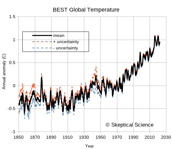
Figure 2: The Berkeley Earth Surface Temperature (BEST) data, including uncertainties. This is typical of the uncertainty estimates by various groups examining global temperature trends.
So, when a new paper comes along that claims that the entire climate science community has been doing it all wrong, and claims that the uncertainty in global temperature records is so large that “the 20th century surface air-temperature anomaly... does not convey any knowledge of rate or magnitude of change in the thermal state of the troposphere”, you can bet two things:
- The scientific community will be pretty skeptical.
- The contrarian community that wants to believe it will most likely accept it without critical review.
We’re here today to look at a recent example of such a paper: one that claims that the global temperature measurements that show rapid recent warming have so much uncertainty in them as to be completely useless. The paper is written by an individual named Patrick Frank, and appeared recently in a journal named Sensors. The title is “LiG Metrology, Correlated Error, and the Integrity of the Global Surface Air-Temperature Record”. (LiG is an acronym for “liquid in glass” – your basic old-style thermometer.)
Sensors 2023, 23(13), 5976
https://doi.org/10.3390/s23135976
Patrick Frank has beaten the uncertainty drum previously. In 2019 he published a couple of versions of a similar paper. (Note: I have not read either of the earlier papers.) Apparently, he had been trying to get something published for many years, and had been rejected by 13 different journals. I won't link to either of these earlier papers here,, but a few blog posts exist that point out the many serious errors in his analysis – often posted long before those earlier papers were published. If you start at this post from And Then There’s Physics, titled “Propagation of Nonsense”, you can find a chain to several earlier posts that describe the numerous errors in Patrick Frank’s earlier work.
Today, we’re only going to look at his most recent paper, though. But before we begin that, let’s review a few basics about the propagation of uncertainty – how uncertainty in measurements needs to be examined to see how it affects calculations based on those measurements. It will be boring and tedious, since we’ll have more equations than pictures, but we need to do this to see the elementary errors that Patrick Frank makes. If all the following section looks familiar, just jump to the next section where we point out the problems in Patrick Frank’s paper.
Spoiler alert: Patrick Frank can’t do basic first-year statistics.
Some Elementary Statistics Background
Every scientist knows that every measurement has error in it. Error is the difference between the measurement that was made, and the true value of what we wanted to measure. So how do we know what the error is? Well, we can’t – because when we try to measure the true value, our measurement has errors! That does not mean that we cannot assess a range over which we think the true measurement lies, though, and there are standard ways of approaching this. So much of a “standard” that the ISO produces a guide: Guide to the expression of uncertainty in measurement. People familiar with it usually just refer to it as “the GUM”.
The GUM is a large document, though. For simple cases we often learn a lot of the basics in introductory science, physics, or statistics classes. Repeated measures can help us to see the spread associated with a measurement system. We are familiar with reporting measurements along with an uncertainty, such as 18.4°C, ±0.8°C. We probably also learn that random errors often fit a “normal curve”, and that the spread can be calculated using the standard deviation (usually indicated by the symbol σ). We also learn that “one sigma” covers about 68% of the spread, and “two sigmas” is about 95%. (When you see numbers such as 18.4°C, ±0.8°C, you do need to know if they are reporting one or two standard deviations.)
At a slightly more advanced level, we’ll start to learn about systematic errors, rather than random ones. And we usually want to know if the data actually are normally-distributed. (You can calculate a standard deviation on any data set, even one as small as two values!, but the 68% and 95% rules only work for normally-distributed data.) There are lots of other common distributions out there in the physical sciences - uniform Poisson, etc. - and you need to use the correct error analysis for each type.
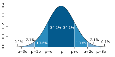
Figure 3: the "normal distribution", and the probabilities that data will fall within one, two, or three standard deviations of the mean. Image source: Wikipedia.
But let’s first look at what we probably all recognize – the characteristics of random, normally-distributed variation. What common statistics do we have to describe such data?
- The mean, or average. Sum all the values, divide by the number of values (N), and we have a measure of the “central tendency” of the data.
- Other common “central tendency” measures are the mode (the most common value) and the median (the value where half the observations are smaller, and half are bigger), but the mean is most common. In normally-distributed data, they are all the same, anyway.
- The standard deviation. Start by taking each measurement, subtracting the mean, to express it as a deviation from the mean.
- We want to turn this into some sort of an “average”, though – but if we just sum up these deviations and divide by N, we’ll get zero because we already subtracted the mean value.
- So, we square them before we sum them. That turns all the values into positive numbers.
- Then we divide by N.
- Then we take the square root.
- After that, we’ll probably learn about the standard error of the estimate of the mean (often referred to as SE).
- If we only measure once, then our single value will fall in the range as described by the standard deviation. What if we measure twice, and average those two readings? or three times? or N times?
- If the errors in all the measurements are independent (the definition of “random”) then the more measurements we take (of the same thing) the close the average will be to the true average. The reduction is proportional to 1/(sqrt(N).
- SE = σ/√N
A key thing to remember is that measures such as standard deviation involve squaring something, summing, and then taking the square root. If we do not take the square root, then we have something called the variance. This is another perfectly acceptable and commonly-used measure of the spread around the mean value – but when combining and comparing the spread, you really need to make sure whether the formula you are using is applied to a standard deviation or a variance.
The pattern of “square things, sum them, take the square root” is very common in a variety of statistical measures. “Sum of squares” in regression should be familiar to us all.
Differences between two systems of measurement
Now, all that was dealing with the spread of a single repeated measurement of the same thing. What if we want to compare two different measurement systems? Are they giving the same result? Or do they differ? Can we do something similar to the standard deviation to indicate the spread of the differences? Yes, we can.
- We pair up the measurements from the two systems. System 1 at time 1 compared to system 2 at time 1. System 1 at time 2 compared to system 2 at time 2. etc.
- We take the differences between each pair, square them, add them, divide by N, and take the square root, just like we did for standard deviation.
- And we call it the Root Mean Square Error (RMSE)
Although this looks very much like the standard deviation calculation, there is one extremely important difference. For the standard deviation, we subtracted the mean from each reading – and the mean is a single value, used for every measurement. In the RMSE calculation, we are calculating the difference between system 1 and system 2. What happens if those two systems do not result in the same mean value? That systematic difference in the mean value will be part of the RMSE.
- The RMSE reflects both the mean difference between the two systems, and the spread around those two means. The differences between the paired measurements will have both a mean value, and a standard deviation about that mean.
- So, we can express the RMSE as the sum of two parts: the mean difference (called the Mean Bias Error, MBE), plus the standard deviation of those differences. We have to square them first, though (remember “variance”):
- σ2 = RMSE2 - MBE2
- Although we still use the σ symbol here, note that the standard deviation of the differences between two measurement systems is subtly different from the standard deviation measured around the mean of a single measurement system.
Combining uncertainty from different measurements
Lastly, we’ll talk about how uncertainty gets propagated when we start to do calculations on values. There are standard rules for a wide variety of common mathematical calculations. The main calculations we’ll look at are addition, subtraction, and multiplication/division. Wikipedia has a good page on propagation of uncertainty, so we’ll borrow from them. Half way down the page, they have a table of Example Formulae, and we’ll look at the first three rows. We’ll consider variance again – remember it is just the square of the standard deviation. A and B are the measurements, and a and b are multipliers (constants).
| Calculation | Combination of the variance |
| f = aA | σf2 = a2 σ2A |
| f=aA+bB | σf2 = a2 σ2A + b2 σ2B + 2ab σAB |
| f=aA-bB | σf2 = a2 σ2A + b2 σ2B - 2ab σAB |
If we leave a and b as 1, this gets simpler. The first case tells us that if we multiply a measurement by something, we also need to multiply the uncertainty by the same ratio. The second and third cases tell us that when we add or subtract, the sum or difference will contain errors from both sources. (Note that the third case is just the second case with negative b.) We may remember this sort of things from school, when we were taught this formula for determining the error when we added two numbers with uncertainty:
σf2 = σ2A + σ2B
But Wikipedia has an extra term: ±2ab σAB, (or ±2σAB when we have a=b=1). What on earth is that?
- That term is the covariance between the errors in A and the errors in B.
- What does that mean? It addresses the question of whether the errors in A are independent of the errors in B. If A and B have errors that tend to vary together, that affects how errors propagate to the final calculation.
- The covariance is zero if the errors in A and B are independent – but if they are not... we need to account for that.
- Two key things to remember:
- When we are adding two numbers, if the errors in B tend to go up when the errors in A go up (positive covariance), we make our uncertainty worse. If the errors in B go down when the errors in A go up (negative covariance), they counteract each other and our uncertainty decreases.
- When subtracting two numbers, the opposite happens. Positive covariance make uncertainty smaller; negative covariance makes uncertainty worse.
- Three things. Three key things to remember. When we are dealing with RMSE between two measurement systems, the possible presence of a mean bias error (MBE) is a strong warning that covariance may be present. RMSE should not be treated as if it is σ.
Let’s finish with a simple example – a person walking. We’ll start with a simple claim:
“The average length of an adult person’s stride is 1 m, with a standard deviation of 0.3 m.”
There are actually two ways we can interpret this.
- Looking at all adults, the average stride is 1 m, but individuals vary, so different adults will have an average stride that is 1 ±0.3 m long (one sigma confidence limit).
- People do not walk with a constant stride, so although the average stride is 1 m, the individual steps one adult takes will vary in the range ±0.3 m (one sigma).
The claim is not actually expressed clearly, since we can interpret it more than one way. We may actually mean both at the same time! Does it matter? Yes. Let’s look at three different people:
- Has an average stride length of 1 m, but it is irregular, so individual steps vary within the ±0.3 m standard deviation.
- Has a shorter than average stride of 0.94m (within reason for a one-sigma variation of ±0.3 m), and is very steady. Individual steps are all within ±0.01 m.
- Has a longer than average stride of 1.06m, and an irregular stride that varies by ±0.3 m.
Figure 4 gives us two random walks of the distance travelled over 200 steps by these three people. (Because of the randomness, a different random sequence will generate a slightly different graph.)
- Person B follows a nice straight line, due to the steady pace, but will usually not travel as far as person A or C. After 200 steps, they will always be at a total distance close to 188m.
- Persons A and C exhibit wobbly lines, because their step lengths vary. On average, person C will travel further than persons A and B, but because A and C vary in their individual stride lengths, this will not always be the case. The further they walk, though, the closer they will be to their average.
- Person A will usually fall in between B and C, but for short distances the irregular steps can cause this to vary.
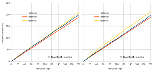
Figure 4: Two versions of a random walk by the three people described in the text. Person A has a stride of 1.0±0.3 m. Person B has a stride of 0.94±0.01 m. Person C has a stride of 1.06±0.3 m.
What’s the point? Well, to properly understand what the graph tells us about the walking habits of these three people, we need to recognize that there are two sources of differences:
- The three people have different average stride lengths.
- The three people have different variability in their individual stride lengths.
Just looking at how individual steps vary across the three individuals is not enough. The differences have an average component (e.g., Mean Bias Error), and a random component (e.g., standard deviation). Unless the statistical analysis is done correctly, you will mislead yourself about the differences in how these three people walk.
Here endeth the basic statistics lesson. This gives us enough tools to understand what Patrick Frank has done wrong. Horribly, horribly wrong.
The problems with Patrick Frank’s paper
Well, just a few of them. Enough of them to realize that the paper’s conclusions are worthless.
The first 26 pages of this long paper look at various error estimates from the literature. Frank spends a lot of time talking about the characteristics of glass (as a material) and LiG thermometers, and he spends a lot of time looking at studies that compare different radiation shields or ventilation systems, or siting factors. He spends a lot of time talking about systemic versus random errors, and how assumptions about randomness are wrong. (Nobody actually makes this assumption, but that does not stop Patrick Frank from making the accusation.) All in preparation for his own calculations of uncertainty. All of these aspects of radiation shields, ventilation etc. are known by climate scientists – and the fact that Frank found literature on the subject demonstrates that.
One key aspect – a question, more than anything else. Frank’s paper uses the symbol σ (normally “standard deviation”) throughout, but he keeps using the phrase RMS error in the text. I did not try to track down the many papers he references, but there is a good possibility that Frank has confused standard deviation and RMSE. They look similar in calculations, but as pointed out above, they are not the same. If all the differences he is quoting from other sources are RMSE (which would be typical for comparing two measurement systems), then they all include the MBE in them (unless it happens to be zero). It is an error to treat them as if they are standard deviation. I suspect that Frank does not know the difference – but that is a side issue compared to the major elementary statistics errors in the paper.
It’s on page 27 that we begin to see clear evidence that he simply does not know what he is doing. In his equation 4, he combines the uncertainty for measurements of daily maximum and minimum temperature (Tmax and Tmin) to get an uncertainty for the daily average:
![]()
Figure 5: Patrick Frank's equation 4.
At first glance, this all seems reasonable. The 1.96 multiplier would be to take a one-sigma standard deviation and extend it to the almost-two-sigma 95% confidence limit (although calling it 2σ seems a bit sloppy). But wait. Checking that calculation, there is something wrong with equation 4. In order get his result of ±0.382°C, the equation in the middle tells me to do the following:
- 0.3662 + 0.1352 = 0.133956 + 0.018225 = 0.152181
- 0.152181 ÷ 2 = 0.0760905
- sqrt(0.076905) = 0.275845065
- 1.96 * 0.275845065 = 0.541
- ...not the 0.382 value we see on the right...
What Frank actually seems to have done is:
- 0.3662 + 0.1352 = 0.133956 + 0.018225 = 0.152181.
- sqrt(0.152181) = 0.3910
- 0.39103832 ÷ 2 = 0.19505
- 1.96 * 0.19505 = 0.382
See how steps B and C are reversed? Frank did the division by 2 outside the square root, not inside as the equation is written. Is the calculation correct, or is the equation correct? Let’s look back at the Wikipedia equation for uncertainty propagation, when we are adding two terms (dropping the covariance term):
σf2 = a2 σ2A + b2 σ2B
To make Frank’s version – as the equation is written - easier to compare, let’s drop the 1.96 multiplier, do a little reformatting, and square both sides:
σ2 = ½ (0.3662)+ ½(0.1352)
The formula for an average is (A+B)/2, or ½ A + ½ B. In Wikipedia’s format, the multipliers a and b are both ½. That means that when propagating the error, you need to use ½ squared, = ¼.
- Patrick Frank has written the equation to use ½. So the equation is wrong.
- In his actual calculation, Frank has moved the division by two outside the square root. This is the same as if he’d used 4 inside the square root, so he is getting the correct result of ±0.382°C.
So, sloppy writing, but are the rest of his calculations correct? No.
Look carefully at Frank's equation 5.
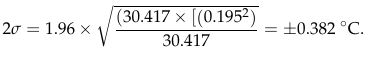
Figure 6: Patrick Frank's equation 5.
Equation 5 supposedly propagates a daily uncertainty into a monthly uncertainty, using an average month length of 30.417. It is very similar in format to his equation 4.
- Instead of adding the variance (=0.1952) for 30.417 times, he replaces the sum with a multiplication. This is perfectly reasonable.
- ...but then in the denominator he only has 30.417, not 30.4172. The equation here is again written with the denominator inside the square root (as the 2 was in equation 4). But this time he has actually done the math the way his equation is (incorrectly) written.
- His uncertainty estimate is too big. In his equation the two 30.417 terms cancel out, but it should be 30.417/30.4172, so that cancelling leaves 30.417 only in the denominator. After the square root, that’s a factor of 5.515 times too big.
And equation 6 repeats the same error in propagating the uncertainty of monthly means to annual ones. Once again, the denominator should be 122, not 12. Another factor of 3.464.
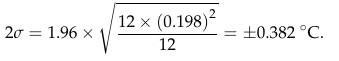
Figure 7: Patrick Frank's equation 6.
So, combining these two errors, his annual uncertainty estimate is √30.417 * √12 = 19 times too big. Instead of 0.382°C, it should be 0.020°C – just two hundredths of a degree! That looks a lot like the BEST estimates in figure 2.
Notice how each of equations 4, 5, and 6 all end up with the same result of ±0.382°C? That’s because Frank has not included a factor of √N – the term in the equation that relates the standard deviation to the standard error of the estimate of the mean. Frank’s calculations make the astounding claim that averaging does not reduce uncertainty!
Equation 7 makes the same error when combining land and sea temperature uncertainties. The multiplication factors of 0.7 and 0.3 need to be squared inside the square root symbol.
![]()
Figure 8: Patrick Frank's equation 7.
Patrick Frank messed up writing his equation 4 (but did the calculation correctly), and then he carried the error in the written equation into equations 5, 6, and 7 and did those calculations incorrectly.
Is it possible that Frank thinks that any non-random features in the measurement uncertainties exactly balance the √N reduction in uncertainty for averages? The correct propagation of uncertainty equation, as presented earlier from Wikipedia, has the covariance term, 2ab σAB. Frank has not included that term.
Are there circumstances where it would combine exactly in such a manner that the √N term disappears? Frank has not made an argument for this. Moreover, when Frank discusses the calculation of anomalies on page 31, he says “the uncertainty in air temperature must be combined in quadrature with the uncertainty in a 30-year normal”. But anomalies involve subtracting one number from another, not adding the two together. Remember: when subtracting, you subtract the covariance term. It’s σf2 = a2 σ2A + b2 σ2B - 2ab σAB. If it increases uncertainty when adding, then the same covariance will decrease uncertainty when subtracting. That is one of the reasons that anomalies are used to begin with!
We do know that daily temperatures at one location show serial autocorrelation (correlation from one day to the next). Monthly anomalies are also autocorrelated. But having the values themselves autocorrelated does not mean that errors are correlated. It needs to be shown, not assumed.
And what about the case when many, may stations are averaged into a regional or global mean? Has Frank done a similar error? Is it worth trying to replicate his results to see if he has? He can’t even get it right when doing a simple propagation from daily means to monthly means to annual means. Why would we expect him to get a more complex problem correct?
When Frank displays his graph of temperature trends lost in the uncertainty (his figure 19), he has completely blown the uncertainty out of proportion. Here is his figure:
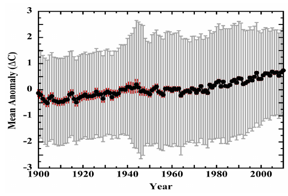
Figure 9: A copy of Figure 19 from Frank (2023). The uncertainties - much larger that those of BEST in figure 2, are grossly over-estimated.
Is that enough to realize that Patrick Frank has no idea what he is doing? I think so, but there is more. Remember the discussion about standard deviation, RMSE, and MBE? And random errors and independence of errors when dealing with two variables? In every single calculation for the propagation of uncertainty, Frank has used the formula that assumes that the uncertainties in each variable are completely independent. In spite of pages of talk about non-randomness of the errors, of the need to consider systematic errors, he does not use equations that will handle that non-randomness.
Frank also repeatedly uses the factor 1.96 to convert the one-sigma 68% confidence limit to a 95% confidence limit. That 1.96 factor and 95% confidence limit only apply to random, normally distributed data. And he’s provided lengthy arguments that the errors in temperature measurements are neither random nor normally-distributed. All the evidence points to the likelihood that Frank is using formulae by rote (and incorrectly, to boot), without understanding what they mean or how they should be used. As a result, he is simply getting things wrong.
To add to the question of non-randomness, we have to ask if Frank has correctly removed the MBE from any RMSE values he has obtained from the literature. We could track down every source Frank has used, to see what they really did, but is it worth it? With such elementary errors in the most basic statistics, is there likely to be anything really innovative in the rest of the paper? So much of the work in the literature regarding homogenization of temperature records and handling of errors is designed to identify and adjust for station changes that cause shifts in MBE – instrumentation, observing methodology, station moves, etc. The scientific literature knows how to do this. Patrick Frank does not.
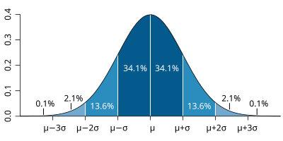
I’m running out of space. One more thing. Frank seems to argue that there are many uncertainties in LiG thermometers that cause errors – with the result being that the reading on the scale is not the correct temperature. I don’t know about other countries, but the Meteorological Service of Canada has a standard operating procedure manual (MANOBS) that covers (among many things) how to read a thermometer. Each and every thermometer has a correction card (figure 6) showing the difference between what is read and what the correct value should be. And that correction is applied for every reading. Many of Frank’s arguments about uncertainty fall by the wayside when you realize that they are likely included in this correction.
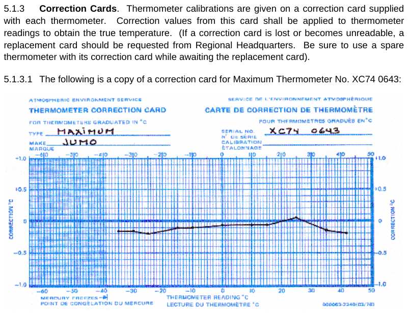
Figure 10: A liquid-in-glass temperature correction card, as used by the Meteorological Service of Canada. Image from MANOBS.
Frank’s earlier papers? Nothing in this most recent paper, which I would assume contains his best efforts, suggests that it is worth wading through his earlier work.
Conclusion
You might ask, how did this paper get published? Well, the publisher is MDPI, which has a questionable track record. The journal - Sensors - is rather off-topic for a climate-related subject. Frank’s paper was first received on May 20, 2023, revised June 17, 2023, accepted June 21, 2023, and published June 27, 2023. For a 46-page paper, that’s an awfully quick review process. Each time I read it, I find something more that I question, and what I’ve covered here is just the tip of the iceberg. I am reminded of a time many years ago when I read a book review of a particularly bad “science” book: the reviewer said “either this book did not receive adequate technical review, or the author chose to ignore it”. In the case of Frank’s paper, I would suggest that both are likely: inadequate review, combined with an author that will not accept valid criticism.
The paper by Patrick Frank is not worth the electrons used to store or transmit it. For Frank to be correct, not only would the entire discipline of climate science need to be wrong, but the entire discipline of introductory statistics would need to be wrong. If you want to understand uncertainty in global temperature records, read the proper scientific literature, not this paper by Patrick Frank.
Additional Skeptical Science posts that may be of interest include the following:
Of Averages and Anomalies (first of a multi-part series on measuring surface temperature change).
Berkeley Earth temperature record confirms other data sets
Are surface temperature records reliable?


[ This will be post #51 , and thus a new page in this thread. ]
Whew ~ I have just finished reading the PubPeer thread of 271 posts.
Which features the Star (Pat Frank) engaging with Paul Pukite, Ken Rice, Joshua Halpern, and Gavin Cawley, in 2019.
Towards the end, Cawley says to Frank : "you are impervious to criticism" and "I have no interest in argument-by-attrition".
And Pukite says (to Frank) "Perhaps worse than being wrong, your paper is just not that interesting and may explain why it was rejected so many times."
Earlier, Rice says (to Frank) : "... you've done a simplistic calculation using a simple model and produced a a result that doesn't represent anything at all."
And that seems to be the heart of it ~ Frank has fired an arrow which has missed the target completely . . . and he spends years wrangling uninsightfully with almost everyone, and insists over & over that they "do not understand physical science". Frank contra mundum.
I won't tax the reader by going into details. The statistics of it all ~ are much less interesting than the personality traits of Dr Frank. Perhaps the most appropriate statistic would be found in the Diagnostic and Statistical Manual [ DSM, Fifth Edition ].
Hello Bob,
Everett F Sargent or Francis F Sargent of ATTP infamy here. I just noticed a Crank reply in the most recent PubPeer article from Frank the Crank ...
https://notrickszone.com/2023/08/24/dr-patrick-franks-refutation-of-a-sks-critique-attempt-loblaws-24-mistakes-exposed/
Now I know that this Crank is wrong although I am not now able to go through the necessary math. Your thoughts on this more recent rebuttal to your post here would be most greatly appreciated. Thanks in advance for your thoughts and/or equations. Also think an abstract of sorts would be most useful covering this crank's misunderstandings from the 2019 and 2023 (this article) papers.
[BL] Since this is your first post here, please note that our Comments Policy does ask that you keep the tone civil. The parts that I have flagged are getting a bit too close to the line.
Hi, ICU/Everett.
I am aware of the PubPeer discussion of this recent Pat Frank paper. I have started participating on that discussion as Camponotus mus - a pseudonym assigned by PubPeer. I saw that link to NoTricksZone, and have a short response waiting in moderation at PubPeer. (As a new, anonymous user at PubPeer, I understand that my comments will always go through moderation, at least for a while.)
I have only looked quickly through that NoTricksZone post, and it seems that Pat Frank is mostly just asserting he is right and the whole world is wrong. Part of my PubPeer response is:
He also seems to claim that uncertainty can't use the rules of statistics, such as the covariance term I mention in the OP. This is certainly a most bizarre idea, as the GUM makes extensive use of statistical models in demonstrating concepts of uncertainty.
Overall, Pat Frank's response at NoTricksZone looks like he is in hagfish mode, as described in DiagramMonkey's blog post. I do not think it would be productive to try to refute it here unless Pat Frank comes here and makes his arguments here. A read-this-blog/read-that-blog cycle will not be at all productive.
Of course, if Pat Frank does come here, he would be expected to follow the Comments Policy, just like anyone else.
ICU @52 , methinks you are asking Bob L to act like Sisyphus.
Sisyphus had a large stone to move to the top of the mountain ~ but Dr Frank's ideas are a much smaller stone (though obviously much denser! ) . . . and the small dense Frankenstein [sorry, the pun was irresistible] is determined to keep rolling itself back down into the gutter [in this case, the gutter press, aka NoTricksZone ] at every opportunity.
As Gavin Cawley says: Frank's methodology is "argument-by-attrition".
Wise psychiatrists know that sometimes you just have to walk away.
On the other hand, Bob may simply enjoy a bit of jousting, for the fun & mental exercise.
Bob,
As I see it, Frank's basic argument is that measurement errors are not random. I think it is better to address the major arguments of a position then to get bogged down in the minutia of an argument.
I would argue that, if in fact, measurement errors are not random, then observational sciences are royally fucked! Meaning, show me explicit examples where the measurement errors are not random and how far those deviate from an assumption of randomness. Actual measurements, not just some made up just so math concoctions.
OK so systematic errors. What specific systematic errors are being claimed for temperature measurements and their magnitude(s)?
ICU: I mentioned the randomness issue briefly above, in the blog post and in comments. He makes the argument for non-randomness saying he finds a non-normal distribution. I point out in comment 46 that he is wrong: you can have non-normal, but still random, distributions.
And he keeps using equations to combine uncertainties that require independence of the variances, which is contrary to his claim of non-randomness. And he uses a multiplier of 1.96 to get 2-sigma from 1-sigma, even though he says that distributions are non-normal.
In the NoTricksZone post, he argues that covariance is not relevant (in fact, that statistics equations combining variances) are not relevant because uncertainty is different from statistics. So he dismisses the equations I have present in the OP - in spite of the fact that they are listed in Wikipedia's "Propagation of Uncertainty" section. Yet covariance is the key concept that needs to be included when things are not random.
In comment 21, bdgwx provided a link to JCGM 100:288, which is basically the same as the 1995 ISO Guide to Uncertainty in Measurement. Section 5.2 talks about Correlated input quantities. If you look at section 5.2.1 on page 33, it says (emphasis added):
The internal inconsistencies in Pat Frank's work are numerous and critical. It's not random, but you don't need to use equations that are designed for correlated inputs. It's not normally-distributed, but you can still get to 95% confidence levels by using the proportions from a normal curve and 1-sigma/2-sigma ratios.
He's picking equations and terms from a buffet based on taste, having no idea how any of the dishes are made, and claiming that he can cook better than anyone else.
In comments 49 and 50, I show data from real world measurements comparing three equivalent temperature sensors, and how you need to properly divide Root Mean Square Error into the Mean Bias Error and standard deviation of differences between pairs to properly evaluate the uncertainty. And how accounting for the Mean Bias Error across sensors (by using anomalies) shows that all three sensors agree on how different the current temperature is from the monthly mean.
Nowhere in Pat Frank's paper does he discuss Mean Bias Error or any other specific form of systematic error. Every single one of his equations ignores the systematic error he claims is a key point.
ICU: I think you posted comment 56 while I was preparing comment 57.
In the OP, the MANOBS chart of temperature correction is an excellent example of systematic error in a temperature sensor - and how to account for it. Here it is again, for convenience.
If this correction is ignored, we see that there is an additional uncertainty of up to 0.2C in the readings - with the exact value depending on temperature. Since each thermometer is calibrated against a better temperatuer sensor (in a lab), we can adjust the reading based on that known systematic error.
But error is not uncertainty... but even if we do not know the error, we can account for any fixed error (e.g., Mean Bias Error) by subtracting each individual reading from the mean (i.e, an anomaly). That fixed error is non-random, so it is present in every reading in the same amount - even if we do not know that amount.
Let me try with a simple equation set: (I know, not that math $#!^ again).
T1true = T1reading + error1
T2true = T2reading + error2
Since we don't know the error (we never can, because anything we compare our reading to also has errors), the unknown is an uncertainty. If error1 and error2 are independent, then all the "combined in quadrature" equations that Pat Frank uses are applicable.
But what if they are related? In the simple case, where the error is completely systematic and fixed (the MBE describes it all), then error1 = error2. In that case when we do T2reading - T1reading, [error2 - error1] = 0, and we get exactly the correct answer for T2true-T1true, even though we have uncertainty in each individual reading.
Comments 49 and 50 demonstrate this using real data. The errors are not purely MBE, but correcting for MBE on a monthly basis greatly reduces the uncertainty.
Much of the literature that Pat Frank references, related to different ventilation shields, different measurement systems, changes in station locations etc., is designed specifically to ferret out the MBE and other systematic errors in temperature measurements. Once that systematic error is identified, it is accounted for through the process of homogenization.
Pat Frank has no idea how any of this actually works.
Dr. Frank not only mixes up evaluations of systemic v random error, but asserts - with no justification - that the extremely statistically durable trends we've found with GAT, sea level, ice melt, etc. have been constructed from systemic errors that, if accounted for, would invalidate them. He has several papers treating these mixes of errors, that all conclude that the trend under discussion is bogus. Again, without even attempts to re-evaluate the data using the "larger" error bounds, and of course also with no treatment of the correlation of these systemic errors. In other words, he ends these papers by throwing up his hands and declaring the data "unevaluable" with zilch for backup.
Bigoilbob @59 :
Yes, very likely that is the ultimate aim of Dr Frank's mathematical contortions ~ to declare all the data to be "unevaluable". That is the desired end-point of the exercise.
Tragic, to have years of effort devoted to "proving" that the mountain of evidence of AGW . . . is non-existent and meaningless. This is the fall-back position of many Denialists ~ though most use a shotgun of poor reasonings, rather than the single bullet approach favored by Dr Frank.
For what it is worth, this recent paper by Pat Frank has received a fair amount of discussion over at PubPeer. Here is the link to that discussion. Note that I have participated using a PubPeer-assigned anonymous user name (Camponotus mus).
Pat Frank did note at PubPeer that he had discovered the inconsistency in the published equation 4, mentioned in the OP here. He said that the calculation (0.382C) is correct, and that the equation should have been written with the 2 in the denominator outside the square root sign. This is what I said would be correct, in the OP. He stands by equations 5 and 6, though.
Equation 4 is not (as of today) corrected in the online version of the paper, or the downloadable PDF. There is a mention of this correction on the web page, if you look in the right margin and find the button labelled "Comment". There is no formal correction notice on the journal page, as far as I can see.
The rest of the PubPeer discussion exposes huge gaps in Pat Frank's understanding of propagation of error, uncertainty, and general statistics. Some of it repeats what I have presented here, but there is some new stuff, too. Warning: head vice required. If you go there, you assume all risks if Pat Frank's hagfishing is too much for you.
Bob Loblaw @61,
I did say up-thread I wasn't going to burrow down into the rabbit holes of Frank's argument. So I haven't look into the references Frank uses to defend his equ 5 & 6. If he were honest about his methods, it should be him explaining why he is right and everybody else wrong. But I note for equ 5 & 6, he only "stands by them."
The nearest Frank comes to an explanation for his equ 5 & 6, for using the RMS for the uncertainty of the combined average of N uncertainties (rather than dividing by N1/2) is found in the first version of nonsense**, Frank (2010). [**Note this is Frank's temperature record nonsense not him climate model nonsense.]
Frank (2010) sets out four 'Cases' for combined uncertainties: 1, 2 3a and 3b. All but Case 3b are as you would expect with the RMS being divided by N1/2 and thus for large combinations, uncertainty will tend to negligable values. But Frank (2010) designates the combination of SAT data as Case 3b for which it says:-
I've not looked to see if the Gleser reference supports such an assertion but it doesn't sound unreasonable although perhaps for the individual variances rather than for the average of those variance.
But Frank then goes on to tell us:-
I have not delved into the reference to see how it would support Frank's assertion. Well, not yet.
MAR:
If the only error or uncertainty is a single, fixed offset that applies to all readings, and there is never any variation at all from that fixed offset, then when adding two numbers with different offsets, the result should be as follows:
In which case you are just simply adding the offsets to get the error. And if you are then dividing the sum by N, the offsets also get divided by N. But you don't go through the gymnastics of squaring and then square-rooting. That is completely redundant. The offsets are not "combined in quadrature", as Pat Frank keep saying.
And if you are dealing with the situation where you are subtracting numbers, say, by calculating anomalies, then a fixed offset means:
..and now you need to compute the difference between the two offsets. And if the offset is so fixed that it is the same for both A and B, then you get the true result for D without having to have any idea at all what that offset is.
Just below equation 6, Pat Frank mentions anomalies, and correctly states that you calculate one by subtracting the monthly mean from the 30-year normal...
...but then he still adds the two offsets together instead of subtracting them. And he does it in the obfuscation of "quadrature".
The form of his equations 5 and 6 is an extreme obfuscation, and only is correct if there is nothing else that affects the errors. And Pat Frank keeps calling it an equation that extends equation 4 (daily uncertainty) into monthly and annual mean temperature uncertainties. He can never give an explanation of what makes equation 4 (as corrected) different from equations 5 and 6.
At PubPeer, he keeps going on about "intrinsic resolution" of liquid-in-glass thermometers, and in the paper he says this about the value coming out of equation 4:
So, is it fixed offset, or a 2σ uncertainty? Only he knows, it seems, and it depends entirely on what argument he is trying to make. Screaming "intrinsic resolution" at the top of his lungs is not a justification for assuming that LiG thermometers only ever have a constant offset with no variation. And fixed errors do not start with "±". Calling it a "±0.382C ... 2σ uncertainty" is the exact opposite of a fixed, unchanging offset.
The Pat Frank Uncertainty Principle seems to be a parallel universe to the Heisenberg Uncertainty Principle. You can tell what he is saying, or what he means, but not both. Things are one thing until Pat Frank says they are something else completely different.
I can only conclude that he is so confused about the issue that he has compartmentalized many different aspects of it, and he can't see the conflicts in his positions. To paraphrase the words of a long-time commenter over at RC "Pat Frank and I have one thing in common. Neither of us has any idea what he is talking about".
Pat Frank's statistics are like Pa Kettle doing basic math. Internally self consistent (in his mind), but...
https://www.youtube.com/watch?v=Bfq5kju627c
One more followup to MAR:
You quote Pat Frank as quoting Giever:
This basically means that you should do what Spock did when calculating the return parameters in Star Trek IV, the Voyage Home.
You can get a more useful discussion n the JCGM 100:2008 mentioned earlier in this thread. In section 4.3, where it discusses "Type B evaluation of standard uncertainty", it says:
In other words, at some point you need to be allowed to make some sort of informed professional judgment.
In no way does it provide justification for Pat Frank's equations 5 and 6. The quote you provide from him is basically word salad that he has used to convince himself of his conclusion.
Bob Loblaw @64,
Having now examined the rabbit hole Frank used to hide the derivation of his equ 5 & 6, I can now say he is flat wrong as he has all along mis-read his reference Bevington & Robinson (2003). (Mind, I'm not sure how he reckons to fit all that Case 3b nonsense into this reference.)
Frank (2020) is saying his reference shows for his Case 3b that varmean = varnoise x (N/(N-1)) with wi=1, indicating the sample uncertainty is a simple average of all the measurement uncertainties vari.
This is a mis-reading of Bevington & Robinson (2003) equ 4.22, the error being that equ 4.22 yields the 'weighted average variance of the data', the varnom from which the individual measurement variances vari are scaled. With wi=1, there is no scaling so the varnom = vari. The actual variance of the mean varmean is given in equ 4.23 where varmean = varnom/N which then yields the division by N1/2 for the standard deviation.
MAR @ 65:
You are trying to ell me that Pat Frank misread and misunderstood something? I'm shocked, I tell you, shocked.
...but you made me go back and read some of Bevington and Robinson again, to try to see what Pat Frank was looking at and why he thinks what he thinks. [I'll forgive you for doing that, this time.]
The odd thing is that the section containing B&R's equation 4.22 is titled "Relative Uncertainties", and follows a section titled "Weighting the data - Nonuniform Uncertainties", and it is all dealing with looking at how to use statistics to determine "the most probably value" and its uncertainty. The everyday mean is "the most probably value" when all points have the same precision, but when they don't, B&R derive equations that account for that.
The B&R section on Relative Uncertainties begins with the statement "It may be that the relative values of σi are known, but the absolute magnitudes are not". And then equation 4.21 is how to estimate a weighted mean, accounting for the ratio between uncertainties. They say (about equation 4.21) that "the result depends only on the relative weights and not on the absolute magnitudes".
And, as you say, B&R then get to equation 4.22 for the "weighted average variance of the data" (not the mean), and equation 4.23 gives the expected 1/sqrt(N) relationship between the σ of the data and the σ of the mean. All this “weighted variance” stuff does not change that 1/sqrt(N) relationship.
But then, as is usual, you try to figure out where the student went wrong and do they deserve part marks, and you realize that all this stuff in this section of B&R is talking about distributions of data where errors are happening randomly. B&R talk about systematic errors as a complication, but the equations presented do not account for that. Pat Frank keeps saying "it's not random, it's systematic". At which point you say "oh, you're looking at equations that don't deal with systematic error".
And then you realize that Pat Frank's equations 4, 5, and 6 are not dealing with relative error - he has specific numbers he has claimed for the uncertainty of maximum and minimum temperature readings, and daily means. In equations 5 and 6 he is claiming that they carry on as constants ad infinitum regardless of averaging period. So you say "you're not looking at equations that should be used when you know the absolute variances".
And then he switches horses and claims that those equations have nothing to do with uncertainty or precision or whatever. He says the 0.382C is not a distribution, etc.
I only see two options:
Some time, over a few beers, I'll have to tell you what I really think.