


 Arguments


A Frank Discussion About the Propagation of Measurement Uncertainty
Posted on 7 August 2023 by Bob Loblaw, jg
Let’s face it. The claim of uncertainty is a common argument against taking action on any prediction of future harm. “How do you know, for sure?”. “That might not happen.” “It’s possible that it will be harmless”, etc. It takes on many forms, and it can be hard to argue against. Usually, it takes a lot more time, space, and effort to debunk the claims than it takes to make them in the first place.
It even has a technical term: FUD.
Acronym of Fear, uncertainty, and doubt, a marketing strategy involving the spread of worrisome information or rumors about a product.
During the times when the tobacco industry was discounting the risks of smoking and cancer, the phrase “doubt is our product” was purportedly part of their strategy. And within the climate change discussions, certain individuals have literally made careers out of waving “the uncertainty monster”. It has been used to argue that models are unreliable. It has been used to argue that measurements of global temperature, sea ice, etc. are unreliable. As long as you can spread enough doubt about the scientific results in the right places, you can delay action on climate concerns.

Figure 1: Is the Uncertainty Monster threatening the validity of your scientific conclusions? Not if you've done a proper uncertainty analysis. Knowing the correct methods to deal with propagation of uncertainty will tame that monster! Illustration by jg.
At lot of this happens in the blogosphere, or in think tank reports, or lobbying efforts. Sometimes, it creeps into the scientific literature. Proper analysis of uncertainty is done as a part of any scientific endeavour, but sometimes people with a contrarian agenda manage to fool themselves with a poorly-thought-out or misapplied “uncertainty analysis” that can look “sciencey”, but is full of mistakes.
Any good scientist considers the reliability of the data they are using before drawing conclusions – especially when those conclusions appear to contradict the existing science. You do need to be wary of confirmation bias, though – the natural tendency to accept conclusions you like. Global temperature trends are analyzed by several international groups, and the data sets they produce are very similar. The scientists involved consider uncertainty, and are confident in their results. You can examine these data sets with Skeptical Science’s Trend Calculator.
So, when someone is concerned about these global temperature data sets, what is to be done? Physicist Richard Muller was skeptical, so starting in 2010 he led a study to independently assess the available data. In the end, the Berkeley Earth Surface Temperature (BEST) record they produced confirmed that analyses by previous groups had largely things right. A peer-reviewed paper describing the BEST analysis is available here. At their web site, you can download the BEST results, including their uncertainty estimates. BEST took a serious look at uncertainty - in the paper linked above, the word “uncertainty” (or “uncertainties”) appears 73 times!
The following figure shows the BEST values downloaded a few months ago, covering from 1850 to late 2022. The uncertainties are noticeably larger in the 1800s, when instrumentation and spatial coverage are much more limited, but the overall trends in global temperature are easily seen and far exceed the uncertainties. For recent years, the BEST uncertainty values are typically less than 0.05°C for monthly or annual anomalies. Uncertainty does not look like a worrisome issue. Muller took a lot of flak for arguing that the BEST project was needed – but he and his team deserve a certain amount of credit for doing things well and admitting that previous groups had also done things well. He was skeptical, he did an analysis, and he changed his mind based on the results. Science as science should be done.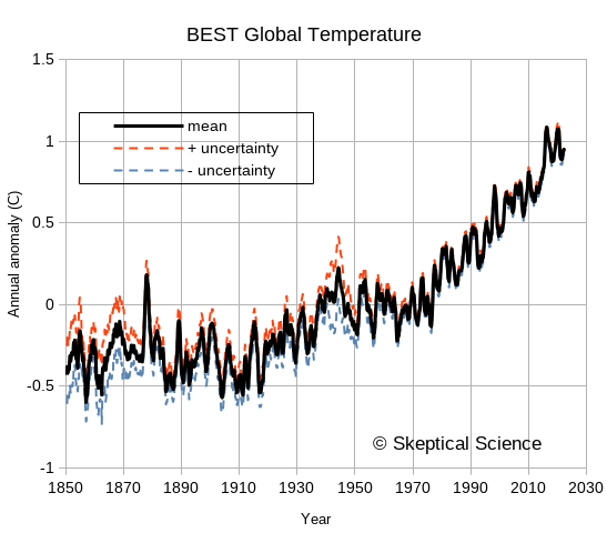
Figure 2: The Berkeley Earth Surface Temperature (BEST) data, including uncertainties. This is typical of the uncertainty estimates by various groups examining global temperature trends.
So, when a new paper comes along that claims that the entire climate science community has been doing it all wrong, and claims that the uncertainty in global temperature records is so large that “the 20th century surface air-temperature anomaly... does not convey any knowledge of rate or magnitude of change in the thermal state of the troposphere”, you can bet two things:
- The scientific community will be pretty skeptical.
- The contrarian community that wants to believe it will most likely accept it without critical review.
We’re here today to look at a recent example of such a paper: one that claims that the global temperature measurements that show rapid recent warming have so much uncertainty in them as to be completely useless. The paper is written by an individual named Patrick Frank, and appeared recently in a journal named Sensors. The title is “LiG Metrology, Correlated Error, and the Integrity of the Global Surface Air-Temperature Record”. (LiG is an acronym for “liquid in glass” – your basic old-style thermometer.)
Sensors 2023, 23(13), 5976
https://doi.org/10.3390/s23135976
Patrick Frank has beaten the uncertainty drum previously. In 2019 he published a couple of versions of a similar paper. (Note: I have not read either of the earlier papers.) Apparently, he had been trying to get something published for many years, and had been rejected by 13 different journals. I won't link to either of these earlier papers here,, but a few blog posts exist that point out the many serious errors in his analysis – often posted long before those earlier papers were published. If you start at this post from And Then There’s Physics, titled “Propagation of Nonsense”, you can find a chain to several earlier posts that describe the numerous errors in Patrick Frank’s earlier work.
Today, we’re only going to look at his most recent paper, though. But before we begin that, let’s review a few basics about the propagation of uncertainty – how uncertainty in measurements needs to be examined to see how it affects calculations based on those measurements. It will be boring and tedious, since we’ll have more equations than pictures, but we need to do this to see the elementary errors that Patrick Frank makes. If all the following section looks familiar, just jump to the next section where we point out the problems in Patrick Frank’s paper.
Spoiler alert: Patrick Frank can’t do basic first-year statistics.
Some Elementary Statistics Background
Every scientist knows that every measurement has error in it. Error is the difference between the measurement that was made, and the true value of what we wanted to measure. So how do we know what the error is? Well, we can’t – because when we try to measure the true value, our measurement has errors! That does not mean that we cannot assess a range over which we think the true measurement lies, though, and there are standard ways of approaching this. So much of a “standard” that the ISO produces a guide: Guide to the expression of uncertainty in measurement. People familiar with it usually just refer to it as “the GUM”.
The GUM is a large document, though. For simple cases we often learn a lot of the basics in introductory science, physics, or statistics classes. Repeated measures can help us to see the spread associated with a measurement system. We are familiar with reporting measurements along with an uncertainty, such as 18.4°C, ±0.8°C. We probably also learn that random errors often fit a “normal curve”, and that the spread can be calculated using the standard deviation (usually indicated by the symbol σ). We also learn that “one sigma” covers about 68% of the spread, and “two sigmas” is about 95%. (When you see numbers such as 18.4°C, ±0.8°C, you do need to know if they are reporting one or two standard deviations.)
At a slightly more advanced level, we’ll start to learn about systematic errors, rather than random ones. And we usually want to know if the data actually are normally-distributed. (You can calculate a standard deviation on any data set, even one as small as two values!, but the 68% and 95% rules only work for normally-distributed data.) There are lots of other common distributions out there in the physical sciences - uniform Poisson, etc. - and you need to use the correct error analysis for each type.
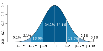
Figure 3: the "normal distribution", and the probabilities that data will fall within one, two, or three standard deviations of the mean. Image source: Wikipedia.
But let’s first look at what we probably all recognize – the characteristics of random, normally-distributed variation. What common statistics do we have to describe such data?
- The mean, or average. Sum all the values, divide by the number of values (N), and we have a measure of the “central tendency” of the data.
- Other common “central tendency” measures are the mode (the most common value) and the median (the value where half the observations are smaller, and half are bigger), but the mean is most common. In normally-distributed data, they are all the same, anyway.
- The standard deviation. Start by taking each measurement, subtracting the mean, to express it as a deviation from the mean.
- We want to turn this into some sort of an “average”, though – but if we just sum up these deviations and divide by N, we’ll get zero because we already subtracted the mean value.
- So, we square them before we sum them. That turns all the values into positive numbers.
- Then we divide by N.
- Then we take the square root.
- After that, we’ll probably learn about the standard error of the estimate of the mean (often referred to as SE).
- If we only measure once, then our single value will fall in the range as described by the standard deviation. What if we measure twice, and average those two readings? or three times? or N times?
- If the errors in all the measurements are independent (the definition of “random”) then the more measurements we take (of the same thing) the close the average will be to the true average. The reduction is proportional to 1/(sqrt(N).
- SE = σ/√N
A key thing to remember is that measures such as standard deviation involve squaring something, summing, and then taking the square root. If we do not take the square root, then we have something called the variance. This is another perfectly acceptable and commonly-used measure of the spread around the mean value – but when combining and comparing the spread, you really need to make sure whether the formula you are using is applied to a standard deviation or a variance.
The pattern of “square things, sum them, take the square root” is very common in a variety of statistical measures. “Sum of squares” in regression should be familiar to us all.
Differences between two systems of measurement
Now, all that was dealing with the spread of a single repeated measurement of the same thing. What if we want to compare two different measurement systems? Are they giving the same result? Or do they differ? Can we do something similar to the standard deviation to indicate the spread of the differences? Yes, we can.
- We pair up the measurements from the two systems. System 1 at time 1 compared to system 2 at time 1. System 1 at time 2 compared to system 2 at time 2. etc.
- We take the differences between each pair, square them, add them, divide by N, and take the square root, just like we did for standard deviation.
- And we call it the Root Mean Square Error (RMSE)
Although this looks very much like the standard deviation calculation, there is one extremely important difference. For the standard deviation, we subtracted the mean from each reading – and the mean is a single value, used for every measurement. In the RMSE calculation, we are calculating the difference between system 1 and system 2. What happens if those two systems do not result in the same mean value? That systematic difference in the mean value will be part of the RMSE.
- The RMSE reflects both the mean difference between the two systems, and the spread around those two means. The differences between the paired measurements will have both a mean value, and a standard deviation about that mean.
- So, we can express the RMSE as the sum of two parts: the mean difference (called the Mean Bias Error, MBE), plus the standard deviation of those differences. We have to square them first, though (remember “variance”):
- σ2 = RMSE2 - MBE2
- Although we still use the σ symbol here, note that the standard deviation of the differences between two measurement systems is subtly different from the standard deviation measured around the mean of a single measurement system.
Combining uncertainty from different measurements
Lastly, we’ll talk about how uncertainty gets propagated when we start to do calculations on values. There are standard rules for a wide variety of common mathematical calculations. The main calculations we’ll look at are addition, subtraction, and multiplication/division. Wikipedia has a good page on propagation of uncertainty, so we’ll borrow from them. Half way down the page, they have a table of Example Formulae, and we’ll look at the first three rows. We’ll consider variance again – remember it is just the square of the standard deviation. A and B are the measurements, and a and b are multipliers (constants).
| Calculation | Combination of the variance |
| f = aA | σf2 = a2 σ2A |
| f=aA+bB | σf2 = a2 σ2A + b2 σ2B + 2ab σAB |
| f=aA-bB | σf2 = a2 σ2A + b2 σ2B - 2ab σAB |
If we leave a and b as 1, this gets simpler. The first case tells us that if we multiply a measurement by something, we also need to multiply the uncertainty by the same ratio. The second and third cases tell us that when we add or subtract, the sum or difference will contain errors from both sources. (Note that the third case is just the second case with negative b.) We may remember this sort of things from school, when we were taught this formula for determining the error when we added two numbers with uncertainty:
σf2 = σ2A + σ2B
But Wikipedia has an extra term: ±2ab σAB, (or ±2σAB when we have a=b=1). What on earth is that?
- That term is the covariance between the errors in A and the errors in B.
- What does that mean? It addresses the question of whether the errors in A are independent of the errors in B. If A and B have errors that tend to vary together, that affects how errors propagate to the final calculation.
- The covariance is zero if the errors in A and B are independent – but if they are not... we need to account for that.
- Two key things to remember:
- When we are adding two numbers, if the errors in B tend to go up when the errors in A go up (positive covariance), we make our uncertainty worse. If the errors in B go down when the errors in A go up (negative covariance), they counteract each other and our uncertainty decreases.
- When subtracting two numbers, the opposite happens. Positive covariance make uncertainty smaller; negative covariance makes uncertainty worse.
- Three things. Three key things to remember. When we are dealing with RMSE between two measurement systems, the possible presence of a mean bias error (MBE) is a strong warning that covariance may be present. RMSE should not be treated as if it is σ.
Let’s finish with a simple example – a person walking. We’ll start with a simple claim:
“The average length of an adult person’s stride is 1 m, with a standard deviation of 0.3 m.”
There are actually two ways we can interpret this.
- Looking at all adults, the average stride is 1 m, but individuals vary, so different adults will have an average stride that is 1 ±0.3 m long (one sigma confidence limit).
- People do not walk with a constant stride, so although the average stride is 1 m, the individual steps one adult takes will vary in the range ±0.3 m (one sigma).
The claim is not actually expressed clearly, since we can interpret it more than one way. We may actually mean both at the same time! Does it matter? Yes. Let’s look at three different people:
- Has an average stride length of 1 m, but it is irregular, so individual steps vary within the ±0.3 m standard deviation.
- Has a shorter than average stride of 0.94m (within reason for a one-sigma variation of ±0.3 m), and is very steady. Individual steps are all within ±0.01 m.
- Has a longer than average stride of 1.06m, and an irregular stride that varies by ±0.3 m.
Figure 4 gives us two random walks of the distance travelled over 200 steps by these three people. (Because of the randomness, a different random sequence will generate a slightly different graph.)
- Person B follows a nice straight line, due to the steady pace, but will usually not travel as far as person A or C. After 200 steps, they will always be at a total distance close to 188m.
- Persons A and C exhibit wobbly lines, because their step lengths vary. On average, person C will travel further than persons A and B, but because A and C vary in their individual stride lengths, this will not always be the case. The further they walk, though, the closer they will be to their average.
- Person A will usually fall in between B and C, but for short distances the irregular steps can cause this to vary.
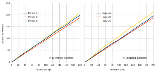
Figure 4: Two versions of a random walk by the three people described in the text. Person A has a stride of 1.0±0.3 m. Person B has a stride of 0.94±0.01 m. Person C has a stride of 1.06±0.3 m.
What’s the point? Well, to properly understand what the graph tells us about the walking habits of these three people, we need to recognize that there are two sources of differences:
- The three people have different average stride lengths.
- The three people have different variability in their individual stride lengths.
Just looking at how individual steps vary across the three individuals is not enough. The differences have an average component (e.g., Mean Bias Error), and a random component (e.g., standard deviation). Unless the statistical analysis is done correctly, you will mislead yourself about the differences in how these three people walk.
Here endeth the basic statistics lesson. This gives us enough tools to understand what Patrick Frank has done wrong. Horribly, horribly wrong.
The problems with Patrick Frank’s paper
Well, just a few of them. Enough of them to realize that the paper’s conclusions are worthless.
The first 26 pages of this long paper look at various error estimates from the literature. Frank spends a lot of time talking about the characteristics of glass (as a material) and LiG thermometers, and he spends a lot of time looking at studies that compare different radiation shields or ventilation systems, or siting factors. He spends a lot of time talking about systemic versus random errors, and how assumptions about randomness are wrong. (Nobody actually makes this assumption, but that does not stop Patrick Frank from making the accusation.) All in preparation for his own calculations of uncertainty. All of these aspects of radiation shields, ventilation etc. are known by climate scientists – and the fact that Frank found literature on the subject demonstrates that.
One key aspect – a question, more than anything else. Frank’s paper uses the symbol σ (normally “standard deviation”) throughout, but he keeps using the phrase RMS error in the text. I did not try to track down the many papers he references, but there is a good possibility that Frank has confused standard deviation and RMSE. They look similar in calculations, but as pointed out above, they are not the same. If all the differences he is quoting from other sources are RMSE (which would be typical for comparing two measurement systems), then they all include the MBE in them (unless it happens to be zero). It is an error to treat them as if they are standard deviation. I suspect that Frank does not know the difference – but that is a side issue compared to the major elementary statistics errors in the paper.
It’s on page 27 that we begin to see clear evidence that he simply does not know what he is doing. In his equation 4, he combines the uncertainty for measurements of daily maximum and minimum temperature (Tmax and Tmin) to get an uncertainty for the daily average:
![]()
Figure 5: Patrick Frank's equation 4.
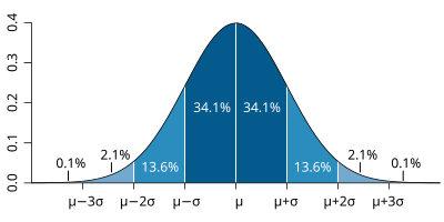
At first glance, this all seems reasonable. The 1.96 multiplier would be to take a one-sigma standard deviation and extend it to the almost-two-sigma 95% confidence limit (although calling it 2σ seems a bit sloppy). But wait. Checking that calculation, there is something wrong with equation 4. In order get his result of ±0.382°C, the equation in the middle tells me to do the following:
- 0.3662 + 0.1352 = 0.133956 + 0.018225 = 0.152181
- 0.152181 ÷ 2 = 0.0760905
- sqrt(0.076905) = 0.275845065
- 1.96 * 0.275845065 = 0.541
- ...not the 0.382 value we see on the right...
What Frank actually seems to have done is:
- 0.3662 + 0.1352 = 0.133956 + 0.018225 = 0.152181.
- sqrt(0.152181) = 0.3910
- 0.39103832 ÷ 2 = 0.19505
- 1.96 * 0.19505 = 0.382
See how steps B and C are reversed? Frank did the division by 2 outside the square root, not inside as the equation is written. Is the calculation correct, or is the equation correct? Let’s look back at the Wikipedia equation for uncertainty propagation, when we are adding two terms (dropping the covariance term):
σf2 = a2 σ2A + b2 σ2B
To make Frank’s version – as the equation is written - easier to compare, let’s drop the 1.96 multiplier, do a little reformatting, and square both sides:
σ2 = ½ (0.3662)+ ½(0.1352)
The formula for an average is (A+B)/2, or ½ A + ½ B. In Wikipedia’s format, the multipliers a and b are both ½. That means that when propagating the error, you need to use ½ squared, = ¼.
- Patrick Frank has written the equation to use ½. So the equation is wrong.
- In his actual calculation, Frank has moved the division by two outside the square root. This is the same as if he’d used 4 inside the square root, so he is getting the correct result of ±0.382°C.
So, sloppy writing, but are the rest of his calculations correct? No.
Look carefully at Frank's equation 5.
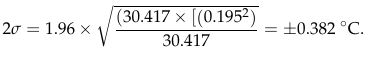
Figure 6: Patrick Frank's equation 5.
Equation 5 supposedly propagates a daily uncertainty into a monthly uncertainty, using an average month length of 30.417. It is very similar in format to his equation 4.
- Instead of adding the variance (=0.1952) for 30.417 times, he replaces the sum with a multiplication. This is perfectly reasonable.
- ...but then in the denominator he only has 30.417, not 30.4172. The equation here is again written with the denominator inside the square root (as the 2 was in equation 4). But this time he has actually done the math the way his equation is (incorrectly) written.
- His uncertainty estimate is too big. In his equation the two 30.417 terms cancel out, but it should be 30.417/30.4172, so that cancelling leaves 30.417 only in the denominator. After the square root, that’s a factor of 5.515 times too big.
And equation 6 repeats the same error in propagating the uncertainty of monthly means to annual ones. Once again, the denominator should be 122, not 12. Another factor of 3.464.
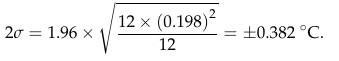
Figure 7: Patrick Frank's equation 6.
So, combining these two errors, his annual uncertainty estimate is √30.417 * √12 = 19 times too big. Instead of 0.382°C, it should be 0.020°C – just two hundredths of a degree! That looks a lot like the BEST estimates in figure 2.
Notice how each of equations 4, 5, and 6 all end up with the same result of ±0.382°C? That’s because Frank has not included a factor of √N – the term in the equation that relates the standard deviation to the standard error of the estimate of the mean. Frank’s calculations make the astounding claim that averaging does not reduce uncertainty!
Equation 7 makes the same error when combining land and sea temperature uncertainties. The multiplication factors of 0.7 and 0.3 need to be squared inside the square root symbol.
![]()
Figure 8: Patrick Frank's equation 7.
Patrick Frank messed up writing his equation 4 (but did the calculation correctly), and then he carried the error in the written equation into equations 5, 6, and 7 and did those calculations incorrectly.
Is it possible that Frank thinks that any non-random features in the measurement uncertainties exactly balance the √N reduction in uncertainty for averages? The correct propagation of uncertainty equation, as presented earlier from Wikipedia, has the covariance term, 2ab σAB. Frank has not included that term.
Are there circumstances where it would combine exactly in such a manner that the √N term disappears? Frank has not made an argument for this. Moreover, when Frank discusses the calculation of anomalies on page 31, he says “the uncertainty in air temperature must be combined in quadrature with the uncertainty in a 30-year normal”. But anomalies involve subtracting one number from another, not adding the two together. Remember: when subtracting, you subtract the covariance term. It’s σf2 = a2 σ2A + b2 σ2B - 2ab σAB. If it increases uncertainty when adding, then the same covariance will decrease uncertainty when subtracting. That is one of the reasons that anomalies are used to begin with!
We do know that daily temperatures at one location show serial autocorrelation (correlation from one day to the next). Monthly anomalies are also autocorrelated. But having the values themselves autocorrelated does not mean that errors are correlated. It needs to be shown, not assumed.
And what about the case when many, may stations are averaged into a regional or global mean? Has Frank done a similar error? Is it worth trying to replicate his results to see if he has? He can’t even get it right when doing a simple propagation from daily means to monthly means to annual means. Why would we expect him to get a more complex problem correct?
When Frank displays his graph of temperature trends lost in the uncertainty (his figure 19), he has completely blown the uncertainty out of proportion. Here is his figure:
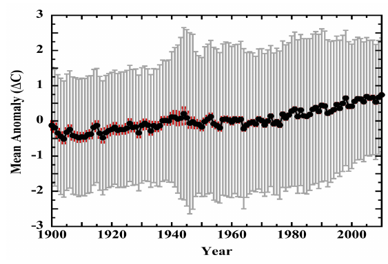
Figure 9: A copy of Figure 19 from Frank (2023). The uncertainties - much larger that those of BEST in figure 2, are grossly over-estimated.
Is that enough to realize that Patrick Frank has no idea what he is doing? I think so, but there is more. Remember the discussion about standard deviation, RMSE, and MBE? And random errors and independence of errors when dealing with two variables? In every single calculation for the propagation of uncertainty, Frank has used the formula that assumes that the uncertainties in each variable are completely independent. In spite of pages of talk about non-randomness of the errors, of the need to consider systematic errors, he does not use equations that will handle that non-randomness.
Frank also repeatedly uses the factor 1.96 to convert the one-sigma 68% confidence limit to a 95% confidence limit. That 1.96 factor and 95% confidence limit only apply to random, normally distributed data. And he’s provided lengthy arguments that the errors in temperature measurements are neither random nor normally-distributed. All the evidence points to the likelihood that Frank is using formulae by rote (and incorrectly, to boot), without understanding what they mean or how they should be used. As a result, he is simply getting things wrong.
To add to the question of non-randomness, we have to ask if Frank has correctly removed the MBE from any RMSE values he has obtained from the literature. We could track down every source Frank has used, to see what they really did, but is it worth it? With such elementary errors in the most basic statistics, is there likely to be anything really innovative in the rest of the paper? So much of the work in the literature regarding homogenization of temperature records and handling of errors is designed to identify and adjust for station changes that cause shifts in MBE – instrumentation, observing methodology, station moves, etc. The scientific literature knows how to do this. Patrick Frank does not.
I’m running out of space. One more thing. Frank seems to argue that there are many uncertainties in LiG thermometers that cause errors – with the result being that the reading on the scale is not the correct temperature. I don’t know about other countries, but the Meteorological Service of Canada has a standard operating procedure manual (MANOBS) that covers (among many things) how to read a thermometer. Each and every thermometer has a correction card (figure 6) showing the difference between what is read and what the correct value should be. And that correction is applied for every reading. Many of Frank’s arguments about uncertainty fall by the wayside when you realize that they are likely included in this correction.
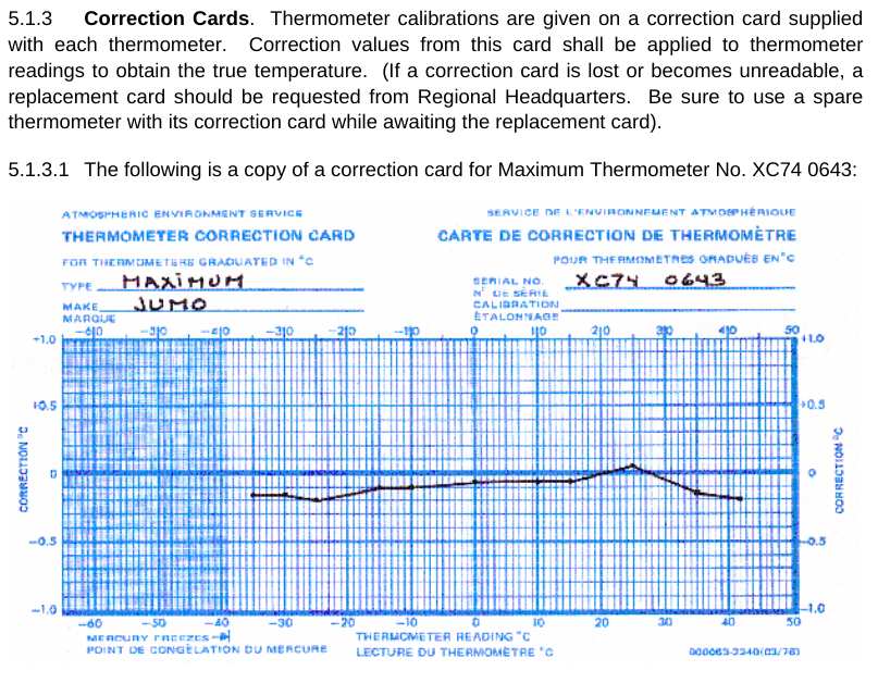
Figure 10: A liquid-in-glass temperature correction card, as used by the Meteorological Service of Canada. Image from MANOBS.
Frank’s earlier papers? Nothing in this most recent paper, which I would assume contains his best efforts, suggests that it is worth wading through his earlier work.
Conclusion
You might ask, how did this paper get published? Well, the publisher is MDPI, which has a questionable track record. The journal - Sensors - is rather off-topic for a climate-related subject. Frank’s paper was first received on May 20, 2023, revised June 17, 2023, accepted June 21, 2023, and published June 27, 2023. For a 46-page paper, that’s an awfully quick review process. Each time I read it, I find something more that I question, and what I’ve covered here is just the tip of the iceberg. I am reminded of a time many years ago when I read a book review of a particularly bad “science” book: the reviewer said “either this book did not receive adequate technical review, or the author chose to ignore it”. In the case of Frank’s paper, I would suggest that both are likely: inadequate review, combined with an author that will not accept valid criticism.
The paper by Patrick Frank is not worth the electrons used to store or transmit it. For Frank to be correct, not only would the entire discipline of climate science need to be wrong, but the entire discipline of introductory statistics would need to be wrong. If you want to understand uncertainty in global temperature records, read the proper scientific literature, not this paper by Patrick Frank.
Additional Skeptical Science posts that may be of interest include the following:
Of Averages and Anomalies (first of a multi-part series on measuring surface temperature change).
Berkeley Earth temperature record confirms other data sets
Are surface temperature records reliable?


He lost me when he called nominal thermometer precision with accuracy. Maybe it was a typo, but such an elementary mistake really takes a toll on any presumed ethos the author may have wanted to project.
You cannot validate science with marketing, nor marketing with scientific processes. In this article there is a lot of taking something hot in one hand as proof the other hand is not cold. A lot of selling going on here.
[BL] - Contents snipped. This is a return of a previously-banned user, using a new name, which is strictly prohibited by the Comments Policy.
Gil @ 1:
Who is "he"? Patrick Frank? Can you specify in which part of his article he makes this reference?
There is a 2017 YouTube presentation by by Dr Patrick T. Brown (climatologist) which is highly critical of Dr Patrick Frank's ideas. The video title is:- "Do 'propagation of error' calculations invalidate climate model projections of global warming?" [length ~38 minutes]
This video currently shows 7235 views and 98 comments ~ many of which are rather prickly comments by Patrick Frank . . . who at one point says "see my post on the foremost climate blog Watts Up With That" [a post in 2015?] # Frank also states: "There's no doubt that the climate models cannot predict future air temperatures. There is also no doubt that the IPCC does not know what it's talking about."
Frank has also made many prickly comments on WUWT at various other times. And he has an acolyte or two on WUWT who will always denounce any critics as not understanding that uncertainty and error are not the same. [And yet the acolytes also fail to address the underlying physical events in global climate.]
In a nutshell : Dr Patrick Frank's workings have a modicum of internal validity mathematically, but ultimately are unphysical.
Yes, Eclectic. That video - and the comments from Pat Frank - are rather mind-boggling. That video is one of the key links given in the AndThenTheresPhysics blog post on Propagation of Uncertainty that I linked to above.
There were many other red flags in the recent paper by Frank. On page 18, in the last paragraph, he makes the claim that "...the ship bucket and engine-intake measurement errors displayed non-normal distributions, inconsistent with random error." There are many other distributions in physics - uniform, Poisson, etc. - that can occur with random data. Non-normality is not a test for randomness.
In this blog post, I focused on the most basic mistakes he makes with respect to simple statistics - standard error of the mean, etc.
Frankly, it is Pat Frank that does not know what he is talking about.
Pat Frank sounds like a classic case of a person promoting crank science. Scientific crank for short.
I'm no expert in scientific cranks, or crank science, but I have a little bit of background in psychology having done a few papers at university, (although I have a design degree). I have observed that cranks have certain attributes.
1)They are usually moderately intelligent, sometimes highly intelligent. This helps them come up with inventive nonsense.
2)They are very stubborn and dont admit they are wrong, either to themselves or anyone else.
3) They also frequently tend to be egocentric, arrogant, very confident and somewhat narcissistic. Some people have a disorder called NPD (narcissistic personality disorder) or lean that way:
"Narcissistic personality disorder is a mental health condition in which people have an unreasonably high sense of their own importance. They need and seek too much attention and want people to admire them. People with this disorder may lack the ability to understand or care about the feelings of others. But behind this mask of extreme confidence, they are not sure of their self-worth and are easily upset by the slightest criticism." (mayo clinic)
Narcissists are usually overconfident and very arrogant and they can sometimes be very dishonest.
We all have some egoism or self love, but narcissists are at the extreme end of the spectrum. Maybe its a bell curve distribution thing.
I've noticed that narcissists are unable to ever admit to themselves or others that they are wrong about something and perhaps its because its exceptionally painful for this personality type. So they just go on repeating the same nonsense forever.
While nobody loves admitting they are wrong, or have been fooled or sucked in, either to themselves or others most people eventually do and move on.
Unfortuntately this means the cranks hang around influencing those who want reasons to deny the climate issue.
And of course some of the scientific cranks prove to be correct at least about some things. Which confuses things further. But it looks to me like most cranks aren't correct, especially the arm chair cranks who may not have science degrees.
The Realclimate.org website attracts some of these cranks, including both climate science denialists and also warmists usually with dubious mitigation solutions. You guys probably know who I mean.
Nigelj @8 , you are correct about some of the characters that you yourself encounter at RealClimate blog. Psychiatrically though, the WUWT blog presents a "target-rich environment" for a wider range of pathologies. And Dr Pat Frank is still to be seen making brief comments in the WUWT threads . . . but mostly his comments match the run-of-the-mill WUWT craziness stuff, rather than relating to the Uncertainty Monster.
Anecdote ~ long ago, I knew a guy who had spent a decade or more tinkering in his garden shed, inventing an electrical Perpetual-Motion machine. Continual updates & modifications, but somehow never quite hitting the bullseye. He had a pleasant-enough personality, not a narcissist. But definitely had a bee in his bonnet or a crack in his pot [=pate]. R.I.P.
And the Uncertainty Monster still lives in the darker corners of public discussion. Living sometimes as a mathematical nonsense, but much more commonly in the form of: "Well, that AGW stuff is not absolutely certain to six decimal places, so we ought to ignore it all." Or existing in the practical sphere as: "It is not certain that we could eventually power all our economy with renewables & other non-fossil-fuel systems . . . so we should not even make a partial effort."
Correction : should be Nigelj @ post 6. Almost certainly!
I'm not sure Frank is responsible for 'propagation' or the spreading of nonsense. He is the creator of nonsense that others happily spread. But strangely the remarkable level of stupidity achieved by Frank and other denialists is not an issue for those who spread such denialist messages, or those who happily receive them.
As for debunking Frank's crazyman attack on climatology, this debunking can be achieved in many ways. There is plenty of opportunity as the man is evidently heavily in denial over AGW and stupid enought to feel he is able to prove that his denial-position is correct while the whole of science is flat wrong.
I'm not of the view that climbing down the rabbit hole to chase his nonsense round down in the wonderland world of Pat Frank is the best way to debunk Fank's lunacy. (I talk of 'chasing his nonsense' because his latest published serving of nonsense is an embellishment of work now a decade-plus old while a whole lot different from his nonsense from four years back featured in the video linked @4.) Yet this SkS OP is attempting such a chase.
Frank's obvious stupidity does lend itself to debunking although his embellishments with lengthy coverage of associated stuff in this 2023 paper provides him a means of obfuscation. In such a situation, I'd go straight for the conclusions, or in Frank's latest paper 'final' conclusions.
So Frank agrees that there has been warming since the 19th century (as shown by phenology which certainly does indicate "unprecedented climate warming over the last 200 years, or over any other timespan" has occurred in recent decades). But generally Frank's paper would suggest the instrument temperature record cannot show any warming. Indeed having told us of the phenological "direct evidence of a warming climate" he then tells us "The 20th century surface air-temperature anomaly, 0.74 ± 1.94 °C (2σ), does not convey any knowledge of rate or magnitude of change in the thermal state of the troposphere." That 0.74 ± 1.94 °C (2σ) surely suggests a 23% chance that measurement of actual temperature represents a cooling not a warming, with a 5% chance of a cooling of -1.2 °C or more.
And really, if anybody were attempting to question the accuracy of the global temperature instrument record, it would be sensible to start with the work already done to establish such accuracy, eg Lenssen et al (2019). But Frank seemingly doesn't do 'sensible'.
Did anyone ever see what the reviewers (including Carl Wunsch and
Davide Zanchettin) said about Frank's similar 2019 paper in Frontiers in Science?
MA Rodger @ 9:
It is an open question whether it is better to ignore papers such as Pat Frank's most recent attempt, or spend the time debunking it. I chose to debunk it in this case, but to paraphrase Top Gun, "this is a target-rich environment". There are so many logical inconsistencies in that 46-page tome that it would take weeks to identify them all. Just trying to chase down the various references he uses would require months of work.
I took this as an opportunity for a "teaching moment" about propagation of uncertainty, as much as an opportunity to debunk Pat Frank. Thanks for the reference to Lenssen et al. But what Pat Frank needs to do is start with a Statistics 101 course.
Nick Palmer @ 10:
I'm sure the general answer to your question is "yes", but I did not try to chase down every blog post and link in the lengthy chain exposed by the linked post at ATTP's. I did read parts of some, and remember that some of his earlier efforts to publish involved open review.
Nigelj's comment that some people "...are unable to ever admit to themselves or others that they are wrong about something..." seems particularly true about Pat Frank.
Eclectic @7, agreed overall.
I didnt mean to imply all cranks are narcissists or lean that way. It just seems to me a disproportionately high percentage of cranks are narcissists. It's just my personal observation but the pattern is rather obvious and striking. I tried to find some research on the issue but without success.
Perhaps the crank tendencies you mentioned and narcissism are mutually reinforcing.
And remember narcissists do frequently come as cross as nice, normal likeable people, just the same as sociopaths (psychopaths) often do. They find this front works best for them. In fact they can be especially likeable, but its about what lies beneath and eventually one notices oddities about them, or in their writings, and if you get into a close relationship with them it can end very badly. Have seen some ciminal cases in the media.
I enjoyed Bob Loblows article because it did a thorough debunking and I learned some things about statistics.
Some of the errors look like almost basic arithmetic and I thought a key purpose of peer review was to identify those things? They did an awful job. It looks like they didnt even bother to try.
Regarding whether such papers should be debunked or not. I've often wondered about this. Given the purpose of this website is to debunk the climate myths it seems appropriate to debunk bad papers like this, or some of them. It would not be possible to address all of them because its too time consuming.
There is a school of thought that says ignore the denialists because "repeating a lie spreads the lie" and engaging with them gives them oxygen. There is some research on this as well. There has to be some truth in the claim that responding to them will spread the lies. It's virtually self evident.
Now the climate science community seems to have taken this advice, and has by my observation mostly ignored the denialists. For example there is nothing in the IPCC reports listing the main sceptical arguments and why they are wrong, like is done on this website (unless Ive missed it). I have never come across any articles in our media by climate scientists or experts addressing the climate denialists myths. The debunking seems to be confined to a few websites like this one and realclimate.org or Taminos open mind.
And how has this strategy of (mostly) giving denialists the silent treatment worked out? Many people are still sceptical about climate change, and progress has been slow dealing with it which suggests that giving the denialists the silent treatment may have been a flawed strategy. I suspect debunking the nonsense, and educating people on the climate myths is more important than being afraid that it would cause lies to spread. Lies will spread anyway.
A clever denialist paper probably potentially has some influence on governments and if its not rebutted this creates a suspicion it might be valid.
However I think that actually debating with denialists can be risky, and getting into actual formal televised debates with denialists would be naieve and best avoided. And fortunately it seems to have been avoided. Denialists frequently resort to misleading but powerful rhetorical techniques (Donald Trump is a master of this) that is hard to counter without getting down into the rhetorical gutter and then this risks making climate scientists look bad and dishonest. All their credibility could be blown with the decision makers.
Nigelj @13,
The paper Frank (2019) did take six months from submission to gain acceptance and Frontiers does say "Frontiers only applies the most rigorous and unbiased reviews, established in the high standards of the Frontiers Review System."
Yet the total nonsense of Frank (2019) is still published, not just a crazy approach but quite simple mathematical error as well.
But do note that a peer-reviewed publication does not have to be correct. A novel approach to a subject can be accepted even when that approach is easily show to be wrong and even when the implications of the conclusions (which are wrong) are set out as being real.
I suppose it is worth making plain that peer-review can allow certain 'wrong' research to be published as this will prevent later researchers making the same mistakes. Yet what is so often lost today is the idea that any researcher wanting publishing must be familiar with the entirety of the literature and takes account of it within their work.
And for a denialist, any publication means it is entirely true, if they want it to be.
In regard to the crazy Frank (2019), it is quite simple to expose the nonsense.
This wondrous theory (first appearing in 2016) suggests that, at a 1sd limit, a year's global average SAT could be anything between +0.35ºC to -0.30ºC the previous year's temperature, this variation due alone to the additional AGW forcing enacted since that previous year. The actual SAT records do show an inter-year variation but something a little smaller (+/-0.12ºC at 1sd in the recent BEST SAT record) but this is from all causes not just from a single cause that is ever accumulating. And these 'all causes' of the +/-0.12ºC are not cumulative through the years but just wobbly noise. Thus the variation seen do not increase with variation measured over a longer period. After 8 years in the BEST SAT record is pretty-much the same as the 1-year variation and not much greater at 60 years (+/-0.22ºC). But in the crazy wonderland of Pat Frank, these variations are apparently potentially cumulative (that would be the logic) so Frank's 8-year variation is twice the 1-year variation. And after 60 years of these AGW forcings (which is the present period with roughly constant AGW forcing) according to Frank we should be seeing SAT changes anything from +17.0ºC to -12.0ºC solely due to AGW forcing. And because Frank's normal distributions provides the probability of these variations, we can say there was an 80% chance of us seeing global SAT increases accumulating over that 60 years in excess of +4.25ºC and/or decreases acumulating in excess of -3.0ºC. According to Frank's madness, we should have been seeing such 60-year variation. But we haven't. So as a predictive analysis, the nonsense of Frank doesn't begin to pass muster.
And another test for garbage is the level of interest shown by the rest of science. In the case of Frank (2019), that interest amounts to 19 citations according to Google Scholar, these comprising 6 citations by Frank himself, 2 mistaken citation (only one by a climatological paper which examines marine heat extremes and uses the Frank paper to support the contention "Substantial uncertainties and biases can arise due to the stochastic nature of global climate systems." which Frank 2019 only says are absent), a climatology working-paper that lists Frank with a whole bunch of denialists, three citations by one Norbert Schwarzer who appears more philosopher than scientist, and six by a fairly standard AGW denier called Pascal Richet. That leaves a PhD thesis citing Frank (2019)'s to say "... general circulation models generally do not have an error associated with predictions"
So science really has no interest in Frank's nonsense (other than demonstrating that it is nonsense).
Bob Loblaw @11
I was interested in what the two reviewers listed actually said. I couldn't find it. Wunsch is highly unlikely to have given it a 5* review and I don't think Zanchettini, who is much less well known, would either.
The reason it would be helpful to know is that Frank's recent '23 paper and its past incarnations, such as '19, are currently being promulgated across the denialosphere as examples of published peer reviewed literature that completely undermines all of climate science. If one knew that Wunsch and Zanchettini had both said seomthing like 'the overall construction of the paper was interesting but has some major logical and statistical flaws in it', and Frontiers in Science had decided to publsih it anyway, that would be very useful anti-denialist 'ammo'.
nigelj @13 wrote " I have never come across any articles in our media by climate scientists or experts addressing the climate denialists myths. The debunking seems to be confined to a few websites like this one and realclimate.org or Taminos open mind"
That's true - but don't forget 'And then there's physics'... and Climate Adam and Dr Gilbz (both phd'd climate scientists) on Youtube quite often debunk stuff. Here's them collaborating - it's fun!
https://www.youtube.com/watch?v=ojSYeI9OQcE
MAR @14. Good points.
Franks "wondrous theory" does indeed sound crazy. What mystifies me is how a guy with a Phd in chemistry, thus very highly scientifically literate could get relatively basic things like that wrong. Because its fairly well doumented that the up and down variation in year to year temperatures is due in large part to a component of natural variability cycles. And he does not seem like a person that would dispute the existence of natural climate cycles.
It makes me wonder if he hasnt actually read much background information like this on the actual climate issue - and perhaps feels he is such a genius that he doesn't need to. Yet this would be astounding really that he is unaware of short term climate cycles and cant see their relevance. I do not have his level of scientific training by a long way, but its obvious to me.
It seems more likely he is he just being crazy about things for whatever reasons and this craziness seems to be the main underling characteristics of a crank. But their frequent narcissim means no matter how much you point out the obvious flaws they just go on repeating the same theories, thus their nonsense certainly compounds over time.
Nigelj @17 :
Cranks or crackpots do inhabit the Denier spectrum, But IMO they are outliers of the main body. Dr Frank's wondrous "Uncertainty" simply produces absurd results ~ see his chart showing the envelope of uncertainty which "explodes" from the observation starting point, rendering all data nearly meaningless. Yet he cannot see the absurdity. He falls back on the bizarre argument of uncertainty being separate from error. (But in practical terms, there is a large Venn Diagram overlap of the two concepts.)
WUWT blog is an enjoyable stamping ground where I observe the denialists' shenanigans. Most of the commenters at WUWT are angry selfish characters, who do not wish to see any socio-economic changes in this world ~ and hence their motivated reasoning against AGW.
Certainly, WUWT has its share of cranks & crackpots. Also a large slice of "CO2-deniers" who continually assert "the trace gas CO2 simply cannot do any global warming". (WUWT blog's founder & patron, Anthony Watts initially tried to oust the CO2-deniers . . . but in the past decade he seems to have abandoned that attempt.)
Dr Frank's comments in a WUWT thread are worth reading, but sadly they rarely rise above the common ruck there. Much more interesting to read, is a Mr Rud Istvan ~ though he does blow his own trumpet a lot (and publicizes his own book "Blowing Smoke" which I gather does in all ways Smite The Heathen warmists & alarmists. Istvan, like Frank, is very intelligent, yet does come out with some nonsenses. For instance, Istvan often states mainstream AGW must be wrong because of reasons A , B , C & D . And unfortunately, 3 of his 4 facts/reasons are quite erroneous. He is so widely informed, that he must know his facts/reasons are erroneous . . . yet he keeps repeating them blindly (in a way that resembles the blindness in Dr Frank).
To very broadly paraphrase Voltaire : It is horrifying to see how even intelligent minds can believe absurdities.
Eclectic @11.
I agree the cranks are a small subset of denilaists and that many of the denialists are fundamentally driven by selfish and economic motives. However you should add political motives to the list, being an ideologically motivated dislike of government rules and regulations. Of course these things are interrelated.
I have a bit of trouble identifying one single underlying cause of the climate denialism issue. It seems to be different denialists have different motives to an extent, randging from vested interests, to political and ideological axes to grind, to selfishness, to just a dislike of change to plain old contrariness. Or some combination. But if anyone thinks there is one key underling motive for the denialim I would be interested in your reasoning.
The cranks are not all deniers as such. Some believe burning fossil fuels is causing warming but some of them think other factors play a very large part like the water cycle or deforestation. A larger part than the IPCC have documented. They unwittingly serve the hard core denialists cause. They are like Lenin and Stalins "useful idiots."
I do visit WUWT sometimes, and I know what you are saying.
"To very broadly paraphrase Voltaire : It is horrifying to see how even intelligent minds can believe absurdities."
Voltaire is right. Its presumably a lot to do with cognitive dissonance. Intelligent minds are not immunue from strong emotively or ideologically driven beliefs and resolving conflicts between those and reality might lead to deliberate ignorance. Reference on cognitive dissonance:
www.medicalnewstoday.com/articles/326738#signs
This does suggests cranks might be driven by underlying belief systems not just craziness.
I meant Eclectic @18. Doh!
I have had numerous discussions with Pat Frank regarding this topic. His misunderstanding boils down to using Bevington equation 4.22. There are two problems here. First and foremost, 4.22 is but an intermediate step in propagating the uncertainty through a mean. Bevington makes it clear that it is actually equation 4.23 that gives you the final result. Second, Equations 4.22 and 4.23 are really meant for relative uncertainties when there are weighted inputs. Frank does not use weighted inputs so it is unclear why he would be using this procedure anyway.
Furthermore, Frank's own source (Bevington) tells us exactly how to propagate uncertainty through a mean. If the inputs are uncorrelated you use equation 4.14. If the inputs are correlated you use the general law of propagation of uncertainty via equation 3.13.
A more modern and robust exploration of the propagation of uncertainty is defined in JCGM 100:2008 which NIST TN 1900 is based.
And I've told Pat Frank repeatedly to verify his results with the NIST uncertainty machine. He has insinuated (at the very least) that NIST and JCGM including NIST's own calculator are not to be trusted.
Another point worth mentioning...he published this in the MDPI journal Sensors. MDPI is known to be a predatory publisher. I emailed the journal editor back in July asking how this publication could have possibly made it through peer review with mistakes this egregious. I basically explained the things mentioned in this article. The editor sent my list of mistakes to Pat Frank and let him respond instead. I was hoping for a response from the editor or the reviewers. I did not get that.
Bdgwx @21 , allow me to say it here at SkS (since I don't post comments at WUWT ) . . . that it is always a pleasure to see your name/remarks featured in the list of comments in any thread at WUWT. You, along with a very small number of other scientific-minded posters [you know them well] provide some sane & often humorous relief, among all the dross & vitriol of that blog.
My apologies for the fulsome praise. ( I am very 'umble, Sir. )
Bdgwx:
Thanks for the additional information. From the Bevington reference you link to, equation 3.13 looks like it matches the equation I cited from Wikipedia, where you need to include the covariance between the two non-independent variance terms. Equations 4.13, 4.14, and 4.23 are the normal Standard Error estimate I mentioned in the OP.
Of course, calculating the mean of two values is equivalent to merging two values where each is weighted by 1/2. Frank's equations 5 and 6 are just "weighted" sums where the weightings are 30.417 and 12 (average number of days in a month, and average number of months in a year), and each day or month is given equal weight.
...and all the equations use N when dealing with variances, or sqrt(N) when dealing with standard deviations. That Pat Frank screws up so badly by putting the N value inside the sqrt sign as a denominator (thus being off by a factor of sqrt(N)) tells us all we need to know about his statistical chops.
In the OP, I linked to the Wikipedia page on MDPI, which largely agrees that they are not a reputable publisher. I took a look through the Sensors web pages at MDPI. There are no signs that any of the editors or reviewers they list have any background in meteorological instrumentation. It seems like they are more involved in electrical engineering of sensors, rather than any sort of statistical analysis of sensor performance.
A classic case of submitting a paper to a journal that does not know the topic - assuming that there was any sort of review more complex than "has the credit card charge cleared?" The rapid turn-around makes it obvious that no competent review was done. Of course, we know that by the stupid errors that remain in the paper.
It is unfortunate that the journal simply passes comments on to the author, rather than actually looking at the significance of the horrible mistakes the paper contains. So much for a rigorous concern about scientific quality.
The JCGM 100:2008 link you provide is essentially the same as the ISO GUM I have as a paper copy (mentioned in the OP).
"Did anyone ever see what the reviewers (including Carl Wunsch and
Davide Zanchettin) said about Frank's similar 2019 paper in Frontiers in Science?"
Carl Wunsch has since disavowed his support for the contents. I'm not sure whether he would have rejected it upon closer reading. Many reviewers want alt.material to be published. If it's good stuff, it will be cited. The 2019 Pat Frank paper and this one have essentially not been...
Bigoilbob @24 , as a side-note :- Many thanks for your numerous very sensible comments in "contrarian" blogsites, over the years. Gracias.
bigoilbob @ 24:
Do you have any link to specific statements from Carl Wunsch? Curiosity arises.
I agree that science will simply ignore the paper. But the target is probably not the science community: it's the "we'll believe ABC [Anything But Carbon]" community, which unfortunately includes large blocks of politicians with significant power. All they need is a thick paper that has enough weight (physical mass, not significance) to survive being tossed down the stairwell, with a sound bite that says "mainstream science has it all wrong". It doesn't matter that the paper isn't worth putting at the bottom of a budgie cage.
"Do you have any link to specific statements from Carl Wunsch? Curiosity arises."
Specifically, this is what I found. Old news, but not to me. I hope that I did not mischaracterize Dr. Wunsch earlier, and my apologies to both him and readers if aI did so.
"#5 Carl Wunsch
I am listed as a reviewer, but that should not be interpreted as an endorsement of the paper. In the version that I finally agreed to, there were some interesting and useful descriptions of the behavior of climate models run in predictive mode. That is not a justification for concluding the climate signals cannot be detected! In particular, I do not recall the sentence "The unavoidable conclusion is that a temperature signal from anthropogenic CO2 emissions (if any) cannot have been, nor presently can be, evidenced in climate observables." which I regard as a complete non sequitur and with which I disagree totally.
The published version had numerous additions that did not appear in the last version I saw.
I thought the version I did see raised important questions, rarely discussed, of the presence of both systematic and random walk errors in models run in predictive mode and that some discussion of these issues might be worthwhile."
https://pubpeer.com/publications/391B1C150212A84C6051D7A2A7F119#5
[BL] Link activated.
The web software here does not automatically create links. You can do this when posting a comment by selecting the "insert" tab, selecting the text you want to use for the link, and clicking on the icon that looks like a chain link. Add the URL in the dialog box.
And here's the twiter thread I began with.
https://twitter.com/andrewdessler/status/1175490719114571776
[BL] Link activated
Thanks, bigoilbob.
That PubPeer thread is difficult to read. The obstinance by Pat Frank is painful to watch.
One classic comment from Pat Frank:
Except, apparently, Pat Frank, who in the paper reviewed above seems to have messed up square rooting the N when propagating the standard deviation into the error of the mean. Unless he actually thinks that non-randomness in errors can be handled by simply dropping the sqrt.
Pat Frank is also quite insistent in that comment thread that summing up a year's worth of a measurement (e.g. temperature) and dividing by the number of measurements to get an annual average gives a value of [original units] per year.
Gavin Cawley sums it up in this comment:
An update. Dr. Frank created an auto erotic self citation for his paper, so there is no longer "no citations" for it.
Diagram Monkey posted about the most recent Pat Frank article.
Thanks for that link, Tom.
I see that DiagramMonkey thinks that I am braver than he is. (There is a link over there back to this post...)
DiagramMonkey's post also has a link to an earlier DiagramMonkey post that has an entertaining description of Pat Frank's approach to his writing (and criticism of it).
DiagramMonkey refers to it as Hagfishing.
DiagramMonkey also has a useful post on uncertainty myths, from a general perspective. It touches on a few of the issues about averaging, normality, etc. that are discussed in this OP.
https://diagrammonkey.wordpress.com/uncertainty-myths/
In the "small world" category, a comment over at AndThenTheresPhysics has pointed people to another DiagramMonkey post that covers a semi-related topic: a really bad paper by one Stuart Harris, a retired University of Calgary geography professor. The paper argues several climate myths.
I have had a ROFLMAO moment reading that DiagramMonkey post. Why? Well in the second-last paragraph of my review of Pat Frank's paper (above), I said:
That was a book (on permafrost) that was written by none other than Stuart Harris. I remember reviewing a paper of his (for a permafrost conference) 30 years ago. His work was terrible then. It obviously has not improved with age.
Here is a lengthy interview with Pat Frank posted 2 days ago.
https://www.youtube.com/watch?v=0-Ke9F0m_gw
Per usual there are a lot of inaccuracies and misrepresentations about uncertianty in it.
[RH] Activated link.
I'm sure this has already been discussed. But regarding Frank 2019 concerning CMIP model uncertainty the most egregious mistake Frank makes is interpretting the 4 W/m2 calibration error of the longwave cloud flux from Lauer & Hamilton 2013 as 4 W/m2.year. He sneakily changed the units from W/m2 to W/m2.year.
And on top of that he arbitrarily picked a year as a model timestep for the propagation of uncertainty even though many climate models operate on hourly timesteps. It's easy to see the absurdity of his method when you consider how quickly his uncertainty blows up if he had arbitrarily picked an hour as the timestep.
Using equstions 5.2 and 6 and assuming F0 = 34 W/m2 and 100 year prediction period we get ±16 K for yearly model timesteps and ±1526 K for hourly model timesteps. Not only is it absurd, but it's not even physically possible.
Bdgwx @36 , you have made numerous comments at WUWT blogsite, where the YouTube Pat Frank / Tom Nelson interview was "featured" as a post on 25th August 2023.
Video length is one hour and 26 minutes long. ( I have not viewed it myself, for I hold that anything produced by Tom Nelson is highly likely to be a waste of time . . . but I am prepared to temporarily suspend that opinion, if an SkS reader can refer me to a worthwhile Nelson production.)
The WUWT comments column has the advantage that it can be skimmed through. The first 15 or so comments are the usual rubbish, but then things gradually pick up steam. Particularly, see comments by AlanJ and bdgwx , which are drawing heat from the usual suspects (including Pat Frank).
Warning : a somewhat masochistic perseverance is required by the reader. But for those who occasionally enjoy the Three-Ring Circus of absurdity found at WUWT blog, it might have its entertaining aspects. Myself, I alternated between guffaws and head-explodings. Bob Loblaw's reference to hagfish (up-thread) certainly comes to mind. The amount of hagfish "sticky gloop" exuded by Frank & his supporters is quite spectacular.
[ The hagfish analogy breaks down ~ because the hagfish uses sticky-gloop to defend itself . . . while the denialist uses sticky-gloop to confuse himself especially. ]
Electic, I appreciate the kind words. I think the strangest part of my conversation with Pat Frank is when he quotes Lauer & Hamilton saying 4 W m-2 and then gaslights me because I didn't arbitary change the units to W m-2 year-1 like he did. The sad part is that he did this in a "peer reviwed" publication. Oh wait...Frontiers in Earth Science is a predatory journal.
Although DiagramMonkey may think that I am a braver person than he is, I would reserve "braver" for people that have a head vice strong enough to spend any amount of time reading and rationally commenting on anything posted at WUWT. I don't think I would survive watching a 1h26m video involving Pat Frank.
I didn't start the hagfish analogy. If you read the DiagramMonkey link I gave earlier, note that a lot of his hagfish analogy is indeed discussing defence mechanisms. Using the defence mechanism to defend one's self from reality is still a defence mechanism.
The "per year" part of Pat Frank's insanity has a strong presence in the PubPeer thread bigoilbob linked to in comment 27 (and elsewhere in other related discussions). I learned that watts are Joules/second - so already a measure per unit time - something like 40-50 years ago. Maybe some day Pat Frank will figure this out, but I am not hopeful.
Oh wow. That PubPeer thread is astonishing. I didn't realize this had already been hashed.
Sorry that this is the first time I have commented have been lurking for years.
Figure 4 3rd explanation
Typo: Person A will usually fall in between A and C, but for short distances the irregular steps can cause this to vary. Should read between B and C.
[BL] Thanks for noticing that! Corrected...
Apart from ATTP's posts on his own website (with relatively brief comments) . . . there is a great deal more in the above-mentioned PubPeer thread (from September 2019) ~ for those who have time to go through it.
So far, I am only about one-third of the way at the PubPeer one. Yet worth quoting Ken Rice [=ATTP] at #59 of PubPeer :-
"Pat, Noone disagrees that the error propagation formula you're using is indeed a valid propagation formula. The issue is that you shouldn't just apply it blindly whenever you have some uncertainty that you think needs to be propagated. As has been pointed out to you many, many, many, many times before, the uncertainty in the cloud forcing is a base state error, which should not be propagated in the way you've done so. This uncertainty means that there will be an uncertainty in the state to which the system will tend; it doesn't mean that the range of possible states diverges with time."
In all of Pat Frank's many, many, many truculent diatribes on PubPeer, he continues to show a blindness to the unphysical aspect of his assertions.
Eclectic # 43: you can write books on propagation of uncertainty - oh, wait. People have. The GUM is excellent. Links in previous comments.
When I taught climatology at university, part of my exams included doing calculations of various sorts. I did not want students wasting time trying to memorize equations, though - so the exam included all the equations at the start (whether they were needed in the exam or not). No explanation of what the terms were, and no indication what each equation was for - that is what the students needed to learn. Once they reached the calculations questions, they knew they could find the correct equation form on the exam, but they needed to know enough to pick the right one.
Pat Frank is able to look up equations and regurgitate them, but he appears to have little understanding of what they mean and how to use them. [In the sqrt(N) case in this most recent paper, he seems to have choked on his own vomit, though.]
Getting back to the temperature question, what happens when a manufacturer states that the accuracy of a sensor they are selling is +/-0.2C? Does this mean that when you buy one, and try to measure a known temperature (an ice-water bath at 0C is a good fixed point), that your readings will vary by +/-0.2C from the correct value? No, it most likely will not.
In all likelihood, the manufacturer's specification of +/-0.2C applies to a large collection of those temperature sensors. The first one might read 0.1C too high. The second might read 0.13C too low. And the third one might read 0.01C too high. And the fourth one might have no error, etc.
If you bought sensor #2, it will have a fixed error of -0.13C. It will not show random errors in the range +/-0.2C - it has a Mean Bias Error (as described in the OP). When you take a long sequence of readings, they will all be 0.13C too low.
Proper estimation of propagation of uncertainty requires recognizing the proper type of error, the proper source, and properly identifying when sampling results in a new value extracted from the distribution of errors.
At the risk of becoming TLDR, I am going to follow up on something I said in comment #5:
Here is a (pseudo) random sequence of 1000 values, generated in a spreadsheet, using a mean of 0.5 and a standard deviation of 0.15. (Due to random variation, the mean of this sample is 0.508, with a standard deviation of 0.147.)
If you calculate the serial correlation (point 1 vs 2, point 2 vs 3, etc.) you get r = -0.018.
Here is the histogram of the data. Looks pretty "normal" to me.
Here is another sequence of values, fitting the same distribution (and with the same mean and standard deviation) as above:
How do I know the distribution, mean , and standard deviation are the same? I just took the sequence from the first figure and sorted the values. The fact that this sequence is a normally-distributed collection of values has nothing to do with whether the sequence is random or not. In this second case, the serial correlation coefficient is 0.99989. The sequence is obviously not random.
Still not convinced? Let's take another sequence of values, generated as a uniform pseudo-random sequence ranging from 0 to 1, in the same spreadsheet:
In this case, the mean is 0.4987, and the standard deviation is 0.292, but the distribution is clearly not normal. The serial correlation R value is -0.015. Here is the histogram. Not perfectly uniform, but this is a random sequence, so we don't expect every sequence to be perfect. It certainly is not normally-distributed.
Once again, if we sort that sequence, we will get exactly the same histogram for the distribution, and exactly the same mean and standard deviation. Here is the sorted sequence, with r = 0.999994:
You can't tell if things are random by looking at the distribution of values.
Don't listen to Pat Frank.
Another interesting aspect of the hypothetical ±0.2 C uncertainty is that while it may primary represent a systematic component for an individual instrument (say -0.13 C bias for instrument A) when you switch the context to the aggregation of many instruments that systematic component now presents itself as a random component because instruments B, C, etc. would each have different biases.
The GUM actually has a note about this concept in section E3.6.
This is why when we aggregate temperature measurements spatially we get a lot of cancellation of those individual biases resulting in an uncertainty of the average that at least somewhat scales with 1/sqrt(N). Obviously there will be still be some correlation so you won't get the full 1/sqrt(N) scaling effect, but you will get a significant part of it. This is in direct conflict with Pat Frank's claim that there is no reduction in the uncertainty of an average of temperatures at all. The only way you would not get any reduction in uncertainty is if each and every instrument had the exact same bias. Obviously that is infintesemially unlikely especially given the 10,000+ stations that most traditional datasets assimilate.
Yes, bdgwx, that is a good point. The "many stations makes for randomness" is very similar to the "selling many sensors makes the errors random when individual sensors have systematic errors".
The use of anomalies does a lot to eliminate fixed errors, and for any individual sensor, the "fixed" error will probably be slightly dependent on the temperature (i.e., not the same at -20C as it is at +25C). You can see this in the MANOBS chart (figure 10) in the OP. As temperatures vary seasonally, using the monthly average over 10-30 years to get a monthly anomaly for each individual month somewhat accounts for any temperature dependence in those errors.
...and then looking spatially for consistency tells us more.
One way to look to see if the data are random is to average over longer and longer time periods and see if the RMSE values scale by 1/sqrt(N). If they do, then you are primarily looking at random data. If they scale "somewhat", then there is some systematic error. If they do not change at all, then all error is in the bias (MBE).
...which is highly unlikely, as you state.
In terms of air temperature measurement, you also have the question of radiation shielding (Stevenson Screen or other methods), ventilation, and such. If these factors change, then systematic error will change - which is why researchers doing this properly love to know details on station changes.
Again, it all comes down to knowing when you are dealing with systematic error or random error, and handling the data (and propagation of uncertainty) properly.
I will not try to say "one last point" - perhaps "one additional point".
The figure below is based on one year's worth of one-minute temperature data taken in an operational Stevenson Screen, with three temperature sensors (same make/model).
The graph shows the three error statistics mentioned in the OP: Root Mean Square Error (RMSE), Mean Bias Error (MBE), and the standard deviation (Std). These error statistics compare each pair of sensors: 1 to 2, 1 to 3, and 2 to 3.
The three sensors generally compare within +/-0.1C - well within manufacturer's specifications. Sensors 2 and 3 show an almost constant offset between 0.03C and 0.05C (MBE). Sensor 1 has a more seasonal component, so comparing it to sensors 2 or 3 shows a MBE that varies roughly from +0.1C in winter (colder temperatures) to -0.1C in summer (warmer temperatures).
The RMSE error is not substantially larger than MBE, and the standard deviation of the differences is less than 0.05C in all cases.
This confirms that each individual sensor exhibits mostly systematic error, not random error.
We can also approach this my looking at how the RMSE statistic changes when we average the data over longer periods of time. The following figure shows the RMSE for these three sensor pairings, for two averaging periods. The original 1-minute average in the raw data, and an hourly average (sixty 1-minute readings).
We see that the increased averaging has had almost no effect on the RMSE. This is exactly what we expect when the differences between two sensors have little random variation. If the two sensors disagree by 0.1C at the start of the hour, they will probably disagree by very close to 0.1C throughout the hour.
As mentioned by bdgwx in comment 47, when you collect a large number of sensors across a network (or the globe), then these differences that are systematic on a 1:1 comparison become mostly random globally.
...and, to put data where my mouth is....
I claimed that using anomalies (expressing each temperature as a difference from its monthly mean) would largely correct for systematic error in the temperature measurements. Here, repeated from comment 49, is the graph of error statistics using the original data, as-measured.
...and if we calculate monthly means for each individual sensor, subtract that monthly mean from each individual temperature in the month, and then do the statistics comparing each pair of sensors (1-2, 1-3, and 2-3), here is the equivalent graph (same scale).
Lo and behold, the MBE has been reduced essentially to zero - all within the range -0.008 to +0.008C. Less than one one-hundredth of a degree. With MBE essentially zero, the RMSE and standard deviation are essentially the same. The RMSE is almost always <0.05C - considerably better than the stated accuracy of the temperature sensors, and considerably smaller than if we leave the MBE in.
The precision of the sensors (small standard deviation) can detect changes that are smaller than the accuracy (Mean Bias Error).
Which is one of the reasons why global temperature trends are analyzed using temperature anomalies.