Lindzen Illusion #2: Lindzen vs. Hansen - the Sleek Veneer of the 1980s
Posted on 29 April 2011 by dana1981
 In 1988, Hansen et al. published a global temperature projection which thus far has turned out to be quite accurate, and yet which numerous "skeptics" have widely criticized and misrepresented. As brought to our attention by Skeptical Science reader Jimbo, noted "skeptic" climate scientist Richard Lindzen gave a talk at MIT in 1989 which we can use to compare to Hansen's projections and see who has been closer to reality over the past two decades. Although to our knowledge Lindzen has never made any specific global temperature projections, he did make some statements in this talk which we can use to extrapolate what his temperature predictions might have looked like.
For example, Hansen and colleagues at NASA Goddard Institute for Space Studies (GISS) began compiling a global surface temperature record (GISTEMP) in 1981. As of 1988–1989, their temperature record showed that the average surface temperature had risen approximately 0.5 to 0.7°C since 1880, when the record begins. Lindzen, however, disputed the accuracy of GISTEMP:
"The trouble is that the earlier data suggest that one is starting at what probably was an anomalous minimum near 1880. The entire record would more likely be saying that the rise is 0.1 degree plus or minus 0.3 degree....I would say, and I don't think I'm going out on a very big limb, that the data as we have it does not support a warming. Whether it contradicts it is a matter of taste"
It turns out that Lindzen's first statement here was incorrect. According to the slightly longer temperature record of the Hadley Centre, 1880 was closer to a local maximum than a minimum. But more importantly, he is claiming here that the average global surface temperature trend between 1880 and 1989 is approximately 0.1°C. Lindzen proceeds to effectively assert that any greenhouse gas warming signal is swamped out by the noise of natural internal variability.
"I personally feel that the likelihood over the next century of greenhouse warming reaching magnitudes comparable to natural variability seems small"
As we recently discussed, natural variability rarely results in more than 0.2 to 0.3°C warming on decadal timescales, so Lindzen is clearly predicting a very small amount of greenhouse warming over the next century. Using these quotes, I reconstructed what I think are two reasonable approximations of global temperature projections based on Lindzen's belief of the small warming effects of greenhouse gases. I want to be explicit that these projections are my interpretation of Lindzen's comments, not Lindzen's own projections.
In both reconstructions, I used the 1880 GISTEMP temperature anomaly (-0.3°C) as the baseline and added some random noise with an amplitude consistent with internal variability (approximately 0.4°C). In the first reconstruction, I then simply added in a linear trend of approximately 0.1°C warming per century.
In the second Lindzen reconstruction, I first calculated, assuming Lindzen's purported 0.1°C warming between 1880 and 1989 were accurate and was caused by CO2 (since the net non-CO2 forcing has been approximately zero), what the climate sensitivity would be, using the following formula and the CO2 levels in 1989 (353 ppm) and pre-industrial (280 ppm):
For a temperature change of 0.1°C, this results in a climate sensitivity parameter (λ) of 0.08 Kelvin per Watts per square meter, or 0.3°C for a doubling of atmospheric CO2. For comparison, the IPCC most likely climate sensitivity value is ten times larger, at 3°C for doubled CO2.
I then used this sensitivity in the same formula above with the annual CO2 levels to add the annual CO2 temperature change to the 1880 baseline plus random noise for Lindzen reconstruction #2.
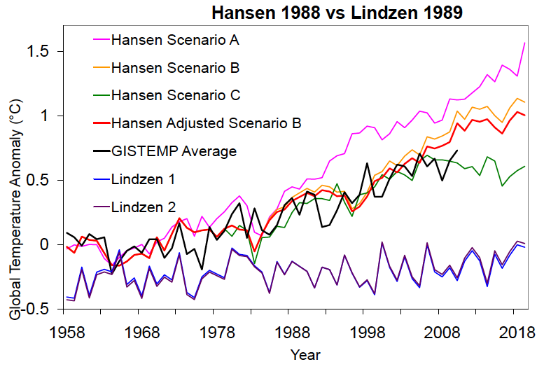
Alongside these reconstructions I also plotted Hansen et al. (1988) Scenarios A, B, and C. As discussed by NASA GISS's Gavin Schmidt, Scenario B was the closest to the actual radiative forcing changes since 1998, but was approximately 10% too high in this regard. Thus I also created an "adjusted" Scenario B to reflect what Hansen's data would have looked like had he correctly projected the greenhouse gas increase.
In the first figure below, these projections are compared to the average of GISTEMP's land and land-ocean temperature records, which may be the most relevant for comparison to Hansen et al. 1988. As in Hansen's original 1988 paper, we begin plotting the data in 1957, and of course as we have previously discussed, GISTEMP is consistent with all the other surface and satellite temperature data sets.

As you can see, Hansen's Scenario B is not far from reality, with a warming trend since 1984 (0.26°C per decade) approximately 30% too high (compared to our average GISTEMP trend of 0.20°C per decade), and the adjusted Scenario B even closer, with a warming trend just 17% higher than observed.
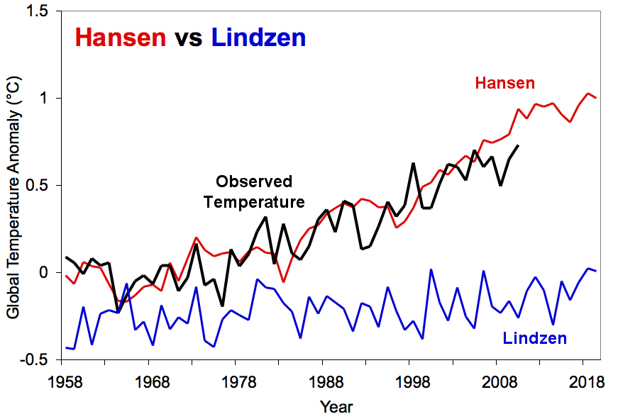
Our reconstructions of Lindzen's projections, on the other hand, increasingly diverge from reality. His warming trend of approximately 0.01°C to 0.02°C per decade is 90 to 95% too low. This is further illustrated in the figure below, which isolates the adjusted Scenario B, our second Lindzen reconstruction, and the GISTEMP average (we have also added this figure to the high resolution climate graphics resource page).

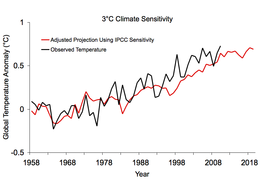
Additionally, Dr. Hansen's 1988 climate model was a bit more sensitive to greenhouse gas changes than the models used by climate scientists today, with a sensitivity of 4.2°C for a doubling of CO2. We can further adjust his Scenario B to reflect the IPCC climate sensitivity of 3°C to determine what today's climate model projections would have looked like in 1988.

As you can see, the projection matches up very well with the observed temperature increase. This supports the IPCC most likely climate sensitivity value of 3°C for doubled CO2.
This analysis demonstrates that Hansen has a record of highly accurate climate projections over the past two decades, while Lindzen has a record of inaccuracy. Indeed, Lindzen continues to argue for low climate sensitivity to this day (not quite as low as 0.3°C, but he continues to argue it's below 1°C for doubled CO2 [i.e. Lindzen and Choi 2009]).
Given all the heat "skeptics" have directed towards Hansen for his projections' slight overestimate of the subsequent warming, one can only wonder what they must think about the massive underestimate of this warming based on Lindzen's 1989 comments.


 Arguments


[DB] You are basing your misinterpretations on a graph. Real life follows physics. Hansen based his modeled projections for the various scenarios (A, B and C) on a climate sensitivity factor that was too high - for each of the scenarios.
Adjustment of the sensitivity to what our current understanding shows it to be yields a much tighter fit to the Scenario B track for actual temperatures than it does for Scenario C. And for down the road, actual emissions diverge widely from the assumptions for Scenario C, so temperatures in the real world will track emissions because of physics, diverging even more widely from those in Scenario C.
You were told all of this before in the thread referenced in comment #35. Why you refuse to understand any of it is beyond me.
[dana1981] Sure, the warming could be natural variation, if you completely ignore all physics and climate science. Just like if I start a forest fire, it could have been started by a lightning strike! Aren't hypotheticals fun?
For your 1°C warming over 100 years claim, I refer you to Monckton Myth #3: Linear Warming.
- Your adjusted Scenario B reduces the projected temperature anomaly for 2019 from 1.10°C to 0.69°C. Wow! This is very close to the Scenario C value of 0.61°C.
- Actual temperatures follow Scenario C much better for the whole period from 1958 to 2010 than your adjusted Scenario B. Your adjusted Scenario B only catches up with Scenario C in 2010. Thereafter it is slightly higher than Scenario C but follows a similar trajectory.

It would appear to be a case of Scenario C - "wrong" physics: right answer. Your adjusted Scenario B - "right" physics: not so good answer. Incidentally, Hansen stated in 1988 Senate Committee hearing that Scenario A is "business as usual". It would appear from your adjusted Scenario B that this was a "massive" overestimate.You already have the post-2000 figures. Scenarios B and C both show a warming trend of 0.26 °C/dec for the 1958-2000 period, however, they diverge post-2000. I show the trends for 2000-2011 here and I summarise them below:
There is a definite dogleg in real world temperatures post-2000.
I request that you publish the figures for the adjusted Scenario B so that I can incorporate them in my models.
[DB] "There is a definite dogleg in real world temperatures post-2000."
The warmest decade in the instrumental record is a "dogleg"? Where's the dogleg:
[Source]
Well, it's not evident in any of the temperature records. How about since 1975 (removing the cyclical noise & filtering out volcanic effects):
[Source]
No dogleg there. How about the warming rate estimated from each starting year (2 sigma error):
[Source]
THe warming since 2000 is significant. Still no dogleg.
Your focus on statistically insignificant timescales is misplaced. While a world-class times-series analyst (like Tamino) can sometimes narrow down a window of significance to decadal scales, typically in climate science 30 years or more of data is used.
I just find it ironic that SkS can praise the accuracy of Hansen's 1988 projections without mentioning the dramatic drop in temperature projections. Here is a timeline derived from SkS blogs for Hansen's 2019 temperature anomaly:
In summary, SkS have presented many blogs praising the accuracy of Hansen (1988) but have neglected to mention that the Hansen's original projection for the 2019 temperature anomaly has plummeted from 1.57°C in 1988 to 0.69°C in Dana (2011). Why is this not mentioned?
Dana, I find it difficult to believe that these plummeting temperatures have not escaped your attention. Do you have a problem with declaring that your adjusted Scenario B is only slightly above Hansen's zero-emissions Scenario C?
Real engineers and scientists use simple models every day to check the validity of their more complex models. They usually use simple physics to check if small changes in their assumptions lead to large changes in outcomes.
Dana in this blog used a simple spreadsheet to adjust Hansen's Scenario B without the need to re-run the whole computer model.
[DB] This has been clarified for you multiple times on several threads. Your persistence and determination in maintaining your narrative in spite of all evidence and physics to the contrary is admirable, but misplaced.
I don't mind continually reinventing the wheel to enable learning, but I draw the line at reinventing the flat tire.
[DB] Accusation of mendacity snipped. You are free to disagree, angusmac. But do not accuse others of lying when it is readily apparent that you either:
In any event, many have wasted their time trying to help you gain a better understanding of the matter. I suggest, if the answers here are not to your liking, a different venue might be in the offing for you to gain the clarity you seek.
[dana1981] You're mistaken. The 0.9 is to account for the fact that the observed radiative forcing (which includes aerosols) is 10% lower than Scenario B.
[dana1981] Because he's trying to exaggerate how far off Hansen was by using this "business as usual" quote, even though it's been explained to him several times that Hansen is not in the business of predicting future CO2 changes.