


 Arguments


SkS Analogy 4 - Ocean Time Lag
Posted on 18 May 2017 by Evan
Tag Line
Greenhouse gases (GHG) determine amount of warming, but oceans delay the warming.
Elevator Statement
To see how the oceans delay warming of the atmosphere, try the following thought experiment.
- Imagine a pot that holds about 8 liters/quarts.
- Hang a thermometer from the center of the lid so that it hangs in the middle of the pot.
- Put the pot on the stove with no water, just air.
- Turn the burner on your stove on very low heat.
- Measure the time it takes for the thermometer to reach 60°C (about 140°F).
- Remove the pot from the stove, let it cool, fill with water, and place it on the stove on very low heat.
- How much longer does it take to reach 60°C (about 140°F) with water instead of air in the pot? A lot longer!
- If you wanted to heat the water to 90°C (about 195°F) in the same amount of time, you would need to start this experiment with the burner on higher heat.
The longer time it takes to heat the pot of water than a pot of air explains why there is a delay between GHG emissions and a rise in temperature of the atmosphere: the oceans absorb a lot of heat, requiring a long time to heat up. This is why scientists such as James Hansen refer to global warming as an inter-generational issue, because the heating due to our emissions are only fully felt by the next generation, due to the time lag created by the oceans.
Climate Science
The earth is covered mostly in water. The large heat capacity of the oceans mean they soak up a lot of energy and slow down the heating of the atmosphere. Just how long is the delay between the time we inject CO2 and other GHG's into the atmosphere and when the effect is felt? The CO2 concentration is like the burner setting in the above example: more CO2 is like a higher burner temperature. However, even though turning up the heat creates hotter water, it takes a while for the water to heat up.
We can estimate the final temperature the atmosphere will reach for a given CO2 concentration by using the average IPCC estimate of 3°C warming for doubling CO2 concentration (this is called the “climate sensitivity”). Using the estimate of pre-industrial CO2 concentration of 280 ppm (parts per million), a climate sensitivity of 3°C implies that CO2 concentrations of 350, 440, and 560 ppm yield 1, 2, and 3°C warming, respectively. Using this estimate of climate sensitivity together with measurements of CO2 from 1970 to today, we can estimate the warming that has been locked in due to recent CO2 emissions. That is, knowing the burner setting, we can estimate the final temperature of the pot of water, even though we will have to wait some time for it to heat up.
We also use the GISS (Goddard Institute for Space Studies) data to plot measured global mean temperature above preindustrial to estimate the time lag between the temperature anomaly suggested by a particular CO2 concentration and the time when that temperature is observed. This and CO2 concentrations for 4 selected years are shown in the following figure.
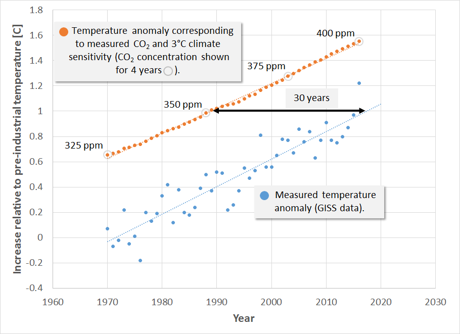
This figure therefore shows the temperature anomaly starting in 1970, the year when the temperature increase due to greenhouse gases began to emerge from the background noise. This figure indicates 3 things: (1) the time lag between emitting greenhouse gases and when we see the principle effect is about 30 years, due mostly to the time required to heat the oceans, (2) the rate of temperature increase predicted by a climate sensitivity of 3°C tracks well with the observed rate of temperature increase, and (3) we have already locked in more than 1.5°C warming. As of 2017 we have reached 406 ppm CO2. At the current increase of 2 ppm CO2/yr., this implies that we will reach 440 ppm and lock in 2°C warming by 2035 … if we don’t act now.
So whereas the experiment at home with a pot of water on low heat yields a time lag of something like 10’s of minutes to heat the water, to heat an Earth-sized pot of water the time lag is about 30 years.
What this figure does not show, however, is that as other complex feedback mechanisms kick in, the rate of warming may begin to exceed the IPCC average climate sensitivity. Therefore, for future trends, this plot likely represents the minimum temperature increase that we can expect for a given CO2 concentration.


How come CO2eq is not used?
I agree with you that CO2eq is the appropriate data to use. However, I have not been able to identify a source to use that melds all of the GHGs together into CO2eq, so for now I am using CO2. Once I identify such a source, I will update the plot in the analogy and begin using CO2eq. I don't think it will change the message, and at most make a small adjustment to the time delay. But I do agree that CO2eq is the appropriate metric to use.
Thanks for pointing this out.
Evan:
This table shows how the most important forcings have changed with time.
If you add all the GHGs, tropospheric aerosols and surface albedo (TA+SA) for each year you will get a time series of man-made forcings from 1850 to 2015. Convert those numbers to "CO2-doublings" by dividing them by 3.96 (the forcing from 2 x CO2 used here) and you can calculate the CO2eq for each year relative to 1850, which had 285.2 ppm CO2 according to this table.
With this approach, I get CO2eq = 416 ppm in 2015 if aerosols and albedo are included, and 513 ppm with GHGs alone.
Thanks HK for the reference. This is great. Just one clarification. I am assuming that the forcings listed in this table increase logarithmicly with CO2 concentration (assuming same relationship between CO2 concentration and ultimate warming). Because this table gives forcings, to convert back to CO2 equivalent I assume that I have to use exponential functions of the ratio of current forcings relative to the forcing at 1850, the date for which we have the reference CO2 concentration.
My calculation of CO2eq from the total man-made forcing in 2015 (excluding sun and volcanoes) was done like this:
Same approach without aerosols and albedo, but the starting point was 3.354 w/m2.
I assumed a constant logarithmic relationship of 3.96 w/m2 per doubling of CO2, but there are probably some very minor changes over that range. The relationship between concentration and forcing for other GHGs are different because they unlike CO2 haven’t achieved band-saturation in the central part of their absorption bands. The forcings of some CFCs are almost linear to their concentrations because they are so rare compared to CO2. There is also a rather complex relationship between CH4 and N2O because their absorption bands partly overlap.
Thanks for the sample HK. So in summary, you are using the same, simple logarithmic relationship that holds for CO2, even though some of the other GHGs have different behavior.
Ravenken, I hope you've learned something from this inquiry and also see why I have not yet woven CO2-eq into any of my plots. I will work on doing that in the future.
Evan:
The behaviour of other greenhouse gases doesn’t matter if you know their forcings beforehand and want to convert them to CO2eq. If the net forcing increases by, say, 1 watt/m2, that can be translated to a ~20% increase of CO2eq regardless of which GHG or combination of GHGs that actually causes this forcing. Therefore, calculating the CO2eq should be relatively straight forward if you know what forcings to include.
Translating a certain forcing to another GHGeq is harder because it requires data about the behaviour of that particular GHG, and they are all different.
BTW, the forcing data I used are available via links on James Hansens site. There you can find both graphs and tables of the forcings as well as concentration data for CO2, CH4, N2O and much more.
Thanks HK for the info and the education. I have a lot of studying to do.
Evan, I have several problems with your graph, and your explanation of it. Starting with the most trivial, when you call 3oC "...the average IPCC estimate..." for the equilibrium temperature response to x2CO2, it is unclear which 'average' you are talking about. To be precise, it is closest to the mean climate sensitivity estimate from the IPCC AR5, which there is good reason to think lies somewhere between 3 and 3.1oC. It is, of course, never explicitly identified by the IPCC. It is significantly higher than the modal (approx 1.8oC) or median (approx 2.55oC) estimates.
That is probably for the good in that if the technique of determining the Equilibrium Climate Sensitivity at x2CO2 illustrated by your graph was valid, then it is essential that your estimate be that which generates the same trend as the observed temperature trend over the period. Your graph does not show that. Indeed, the best fit to the current observed temperature trend since 1970 is for a climate sensitivity of 2.85oC per doubling of CO2.
More troubling is that that value generates a 'lag' of 21 years, although the precise value is sensitive to how you baseline the "preindustrial" temperature. I used the mean of the first 30 years of the temperature record. Had I added the best estimate 0.2oC for the difference between the 1736-1765 mean and the 1880-1909 mean, the lag would have reduced to 10 years.
Further, the lag can only properly be interpreted for a climate sensitivity that exactly generates the observed temperature trend. For other climate sensitivities, because of the difference in trends the lag will differ at different time intervals. Taken at 1970, the IPCC likeley (ie, 67% confidence interval) range of climate sensitivities generates lags from 6 to more than 39 years using the 1880-1909 baseline. The lower bound of a hypothetical 90% confidence interval (1oC) generates a lag of -3 years using your method of determination. (Note, it is a hypothetical 90% confidence interval because the IPCC do not give the upper bound, instead giving the upper bound of a hypothetical 80% confidence interval, ie, 6oC.)
These problems arise because the temperature response is not just a response to the forcing a given number of years ago, no matter what the interval. If the forcing changed in a single pulse, and remained constant after that change, then indeed the temperature would change over time as a response to that pulse. It would increase rapidly at first, with the temperature increase slowing over time until equilibrium was reached. With the actual, gradual increase in forcing, the temperature change in a given year being a consequence of the change in forcing in all preceding years out to a time horizon of potentially several centuries. This is well illustrated by Kevin Cowtan's two box model (see also And Then There's Physics.)
This means that the implicit physics of your graph is wrong. It does not indicate (ie, demonstrate) either the time lag or the equilibrium climate sensitivity. And taken as an analogy, it confuses rather than illuminates.
Thanks for the input Tom.
I would argue that the difference between 2.85 and 3.0 is minor. You and I are fairly well educated on these matters so I can follow you arguments (I model particle formation in chemical reactors), but the analogies are mostly written for people who have never thought about the effect of the oceans. The time lag of 20, 30, or more years includes many more complex physics, as you point out, but the salient point is that there is a decadal-scale time lag between what we do and when when see the effect, and for my intented audience, that is already news.
But thank you very much for the additional information you provided.
With your water pot analogy, I don't understand how heating from below the water is equivalent to atmospheric warming. With GHGs the atmosphere is warming, where the thermometer is, so the heat would be forced down into the pot and there would be no lag. What am I getting wrong here?
No matter where the heat comes from, there will be a lag between the time you apply the heat, and the time at which you see the water heat up to a certain level, as indicated by the thermometer. If the thermometer is in the water, and the heat comes from above, the heat from above still has to warm up the water. Until the water warms up, the thermometer will not respond.
Does that make sense?