Posted on 1 February 2022 by Bob Loblaw

We occasionally receive excellent questions and/or comments by email or via our contact form and have then usually corresponded with the emailer directly. But, some of the questions and answers deserve a broader audience, so we decided to highlight some of them in a new series of blog posts.

An individual recently emailed the Skeptical Science team, asking for comments on a 2012 journal paper that raises questions about the causes of global temperature changes over the last century. The conclusions of the paper differ significantly from most of the literature covering the global temperature trends of the past century. That may give reason to be skeptical of the result, but we can’t dismiss the paper simply on the basis of disagreeing with the conclusions. Any reasonable paper deserves to have someone look at the entire paper – the data used, the methodology in the analysis, the interpretation of the results – to see if the conclusions are justified based on the information provided. (Spoiler alert: I don’t think they are.)

Although the paper concludes that the largest contribution to the 20th century warming comes from anthropogenic sources, it argues that the total solar contribution is larger than values that are usually found in most of the climate literature. The emailer pointed out that paper has a small number of citations [Google Scholar says 21] and is not cited in the IPCC reports, and the emailer wondered if the Skeptical Science team knew of any scientific errors in the paper. This led the Skeptical Science team to obtain the paper and examine it. and this blog post is the result. (Spoiler alert: yes, we think the paper has problems.)

The paper in question is the following:

Shlomi Ziskin, Nir J. Shaviv, "Quantifying the role of solar radiative forcing over the 20th century”, Advances in Space Research, Volume 50, Issue 6, 2012, Pages 762-776

https://www.sciencedirect.com/science/article/abs/pii/S0273117711007411

https://doi.org/10.1016/j.asr.2011.10.009

The paper is part of a special issue titled “Solar Variability, Cosmic Rays and Climate“. This collection of papers appeared at a time when there was a lot of speculation about the role of cosmic rays and such on global temperature trends. The issue starts with an editorial by the editor titled "Solar Variability, Cosmic Rays and Climate: What’s up?". In his opening sentence, he refers to it as "an acute and hotly debated topic." We are only going to examine the Ziskin and Shaviv paper here, but this overall context of the science at the time is worth remembering.

Although the publisher’s web site is pay-walled (only the abstract is freely available), a web search finds links to free copies.

This post digs more deeply into the paper, and we’ll discuss several aspects of the methodology and analysis that severely weaken the argument. While we are at it, we will cover some general information about simple climate models, climate forcings, and model fitting – all of which pertain to the Ziskin and Shaviv paper.

What Ziskin and Shaviv present

The Ziskin and Shaviv paper uses the National Climate Data Center (NCDC) observed global land surface and sea surface temperatures series (LST, SST), and then fits the data using a simple energy balance model (EBM). The EBM has three coupled boxes that can store and exchange energy: a land component, an ocean mixed layer component (the shallow ocean that interacts with the atmosphere, taken to be 75 m deep), and a deep ocean component (taken to extend to 400 m). The land and shallow ocean components are quantified using a single temperature each (changing over time), which is compared to the observed LST and SST from 1880 to 2000. The deep ocean box is thermally linked to the shallow ocean through a diffusion equation, but modelled deep ocean temperatures are not compared to any observations.

The land and mixed layer boxes respond to climate forcing parameters and exchange energy with each other. The deep ocean box only exchanges energy with the ocean mixed layer box. (Energy has to move through the ocean mixed layer to get in our out of the deep ocean.) The different heat capacities and thermal diffusion characteristics in the three boxes will lead to different response times and time lags as the forcing parameters change over time.

Figure 1 and equations 1-5 in Ziskin and Shaviv describe the model details. For convenience and discussion, we reproduce their figure 1 here.

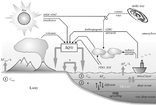
Figure 1: a diagram of Ziskin and Shaviv's energy balance model (reproduced from figure 1 of their paper).

In order to drive the energy moving into the EBM, Ziskin and Shaviv use a catch-all “forcing function” that combines several known and a few speculative components. They include greenhouse gases (GHGs), solar output (as indicated by Total Solar Irradiance, TSI), direct stratospheric and tropospheric aerosols, and an indirect aerosol effect. They then add some uncommon ones: an indirect solar effect (ISE) that they suggest can account for solar effects not included in the TSI, and two factors that normally represent internal variability: the Pacific Decadal Oscillation (PDO) index and Southern Oscillation Index (SOI). (They also tried the North Atlantic Oscillation (NAO) index, but decided not to include it in the final analysis.)

In order to move energy out of the model, they also include an infrared radiation loss term, and diffusion of heat into the deep ocean.

The main forcing factors – GHGs, TSI, direct aerosol effects - are variables that are all well-described in physics and give direct forcing values in W/m². These can be used directly in Ziskin and Shaviv’s “forcing function”. The remaining terms are not energy terms, and the values that Ziskin and Shaviv use to represent these factors need to be converted into W/m² using coefficients that cannot be determined using any known physics. Ziskin and Shaviv allow these coefficients to vary over a range (their table 2), and let the model fitting process determine the best fit values. In addition, the model fitting processes is allowed to change coefficients that affect the energy exchange between the boxes (land, shallow ocean, deep ocean), the initial box temperatures, the box temperatures that correspond to zero radiative forcing, and a “gain” parameter that affects the entire “forcing function” and serves as an adjustment for overall climate sensitivity.

In total, Ziskin and Shaviv’s table 2 lists 11 free parameters that are used in fitting their model. The fitting process minimizes the temperature residuals – the difference between the observed LST and SST values from NCDC and the modelled results for the land and shallow ocean boxes.

My initial reaction is “11 free parameters? That’s an awful lot”. I am reminded of the famous von Neumann quote “With four parameters I can fit an elephant, and with five I can make him wiggle his trunk”. With 11 parameters, Ziskin and Shaviv should be able to get the elephant to paint their house. There is a severe risk of over-fitting here, and we need to question whether all these free parameters are independent.

Ziskin and Shaviv  then present the results of their fitting process – done by performing simulations with a wide range (their table 2) of the free parameters in the model, looking for an optimal fit. They then examine the probability distribution functions (PDFs) of the model fit parameters – essentially looking at whether they find a wide or narrow range of “best fit” values for each parameter, over many model simulations. (They change the fit by reducing the data fed into the model - essentially, providing it with a subset of the full data.)  A narrow range for a fitted parameter is taken as an indication that it can be reliably estimated. They end up concluding that their indirect solar effect (ISE) is an important new feature that represents some undiscovered and undetermined process whereby the sun contributes to recent warming. (Spoiler alert: it probably does not.)

To examine where Ziskin and Shaviv’s argument breaks down, we need to take a bit of time to discuss simple EBMs, climate forcing, and model fitting. Tangent at hand, let us now take a bit of time to cover some general principles, and then come back to Ziskin and Shaviv.

Simple Energy Balance Models and Climate Forcing

There is nothing intrinsically wrong with simple energy balance models. Heck, people have even written books on the subject, such as North and Kim’s Energy Balance Climate Models. The flavour of model used by Ziskin and Shaviv is very similar to the class of "box" models discussed back in 2011 by Isaac Held at this NOAA web page.

You do need to understand their limitations, though – and their limitations are usually linked to the character of the input data that they use and how they handle internal processes. A big question is whether these model components follow fairly rigorous physics, or whether parameters or processes are simply statistical curve-fitting. We are probably all familiar with coefficients that get labelled using terms such as “Fudge Factor”, “Finnegan’s Finagling Factor”, or “Cook’s Constant” - all of which can loosely be defined as “the ratio between the answer I got and the answer I wanted”. Are we discovering something real, or are we fitting an elephant?

So, let’s start with the simplest of all energy balance climate models – the zero-dimensional equilibrium model, where energy absorbed from solar radiation is balanced by an equal emission of infrared radiation determined from the Stefan-Boltzman equation:

 S = σT⁴                               (1)

 where

• S is the absorbed solar radiation.
• For a solar irradiance of 1368 W/m², and an earth albedo (reflectivity) of 0.3, and accounting for a factor of 4 (earth’s spherical surface area vs. the area of the 2-d circle that intercepts sunlight), we get S=239.4 W/m².
• σ is the Stefan-Boltzman constant, 5.67 x 10^-8.
• T is the effective radiating temperature of the earth-atmosphere system, in Kelvin.

This is the commonly-used simple model that gives us a global temperature of about 255K. (Of course, this is the effective IR temperature as seen from space, not the surface temperature.)

For this model, the external forcing is S. The temperature T is an internal model parameter that can vary in response to changes in S. What can we do with this model? Not much – we have one variable controlled by external physics (S), and one free parameter that we can change (T) to meet the requirement that the two sides of the equation balance. As we change S, simple algebra allows us to solve for the internal temperature, T.

We could use this to estimate how T will change if we change S:

• If the new forcing becomes S+4,
• ...the new equilibrium T will become about 256K, for a warming of 1 K (or 1 C°).

This model tells us nothing about how long it will take to warm, though. It will not be instantaneous. The model has no terms that allow it to handle changing temperature over time, or a non-equilibrium state where absorbed solar radiation does not balance with emitted IR. In order to look at changes in temperature with time, we need to add to our model so that it has terms for that process. This is not that difficult. We can write a new model as follows:

ΔT/C = S – σT⁴                               (2)

where ΔT is the rate of temperature change with time, and C is the heat capacity of the earth-atmosphere system. Both sides of the equation need to match in units. The right side is in W/m², and ΔT is in K per unit time, so the heat capacity, C, needs to be in (K/time)/(W/m²). Since W = J/second, if we express ΔT in K/second, the seconds cancel out and we get C in K/(J/m²). – i.e., C tells us how much energy it takes to raise a one square metre column of the earth-atmosphere system by one K. Our new model incorporates the old equilibrium model: if S = σT⁴, then the right side equals zero and the left side must also equal zero, which means temperatures are not changing. When S ≠σT⁴, though, the new model allows us to estimate the rate of temperature change (as long as we have a reasonable estimate of C).

We need to be very careful how we specify a climate change forcing in our new model though. In our first equation, we called S the forcing. When discussing climate change, however, it is more common to use the term “forcing” to describe the change that is pushing climate away from its normal equilibrium state. Wikipedia has a good page on “radiative forcing”. This change creates an imbalance between inputs and outputs, and the system (either the model or the real world) will need to respond to that change.

In our second model, the imbalance is not the 4 W/m² we added to S; it is the difference between absorbed solar (S+4) and the emitted IR (σT⁴) – the right hand side of our model. The imbalance starts at 4 W/m² when we first increase S, but it decreases over time – reaching zero as the new equilibrium is reached.

Let’s look at how our second model simulates temperature over time, using two scenarios:

• In one, we will add 4 to the value of S at time step 100, and let the imbalance (S – σT⁴) change as the temperature responds. This scenario is labelled (S+4) in figure 2.
• In the second, we will specify a permanent imbalance of 4 W/m² – i.e., (S–σT⁴) = 4 W/m². This scenario is labelled (S–σT⁴ = 4) in figure 2.
• We will run both simulations out for 1000 time steps.

Figure 2 gives the temperature versus time for these two simulations. The key features are:

• In the (S+4) case, we see that the temperature first begins to rise rapidly, but slows as the increase in emitted IR compensates for the higher solar input. It stabilizes at about 256K – which is what we predicted from our first model that only describes equilibrium conditions.
• In the (S–σT⁴ = 4) case, we see a very different behaviour. Since we are continuously adding 4 W/m², we see a continuous temperature rise. Even though σT⁴ rises over time, we are constantly increasing S over time so that (S – σT⁴) is always 4 W/m².

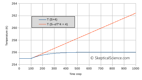
Figure 2. Temperature change with time for our simple zero-dimensional model, after an increase in forcing at time step 100. In the simulation one time step is one day, and the heat capacity in equation 2 corresponds to the atmosphere only. See the text for an explanation of the labels (S+4) and (S–σT⁴ = 4).

Figure 3 shows the components of the imbalance, (S – σT⁴) for the two simulations. For the first 100 times steps, the imbalance is zero (our initial equilibrium at 255K). At step 100, the imbalance jumps to +4 W/m², in both simulations. As soon as the temperature starts to rise, the imbalance drops in the (S+4) simulation, but it stays at +4 W/m² in the (S–σT⁴ = 4) simulation. The figure also includes the change in the σT⁴ term. For the first 100 time steps, σT⁴ is unchanged from the value for 255K (so our graph shows zero). As temperature rises, outgoing IR increases until the temperature reaches 256K and outgoing IR has increased by 4 W/m² - matching our increase in S.

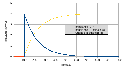
Figure 3. The radiative imbalance for the two simulations given in figure 2.

Which way is correct? The (S+4) scenario? Or the (S–σT⁴ = 4) scenario? Well, “correct” depends on what you are trying to simulate. In our case, we want to simulate increasing S by 4, and let the climate adjust to that new value as temperature rises until σT⁴ re-balances the forcing. The (S+4) scenario does this properly, since the changes in the σT⁴ term do not lead to any changes in S - i.e., there is no feedback from T to our S value. If such a feedback existed (e.g. albedo changes, which we have assumed are constant when we calculated S), then a scenario similar to (S–σT⁴ = 4) might make sense, but the feedback in our (S–σT⁴ = 4) is too strong to be realistic.

What do we conclude from this? Well, the way we handle inputs to the model must be consistent with the way that the model treats that input. If our  model bundles terms together, they must all be treated the same way. No mixing and matching, or our model becomes unrealistic.

Now that we have finished this tangent on simple energy balance models and climate forcing, we can get back to looking at the details of the Ziskin and Shaviv paper.

Climate forcing in the Ziskin and Shaviv paper

In our tangent on EMS and climate forcing, we saw that it is important to recognize the difference between two approaches to modelling:

• An approach that specifies just the radiation input changes (e.g., solar) directly, and allows the earth-atmosphere system to compensate within the model by increasing the IR losses on its own (σT⁴).
• An approach that specifies the imbalance between gains and losses (our S–σT⁴ = 4 scenario), and does not explicitly include the IR losses (σT⁴) as a term in the model.

Either approach can work, but it is essential that you pick one or the other and stick to it. From what I see in the Ziskin and Shaviv paper, they do not. Here is what I read from the paper:

• Ziskin and Shaviv do have a term that includes the IR losses to space, but it is not that easy to see. (I missed it until someone else on the Skeptical Science team pointed it out to me while we were discussing the paper. That's why we are a team.)
• They do not include the Stefan-Boltzman equation explicitly (σT⁴).
• Equations 1 and 2, and figure 1, do include terms that subtract (1/λ)*ΔT for each of land/ocean boxes.
• The λ term is the climate sensitivity - the ratio between radiative temperature and IR emission.
• The ΔT term is the temperature anomaly - the current temperature at each time in the model compared to the normal equilibrium temperature.
• Note that this normal equilibrium temperature is one of their free parameters - "land/mixed ocean temperature at 0 radiative forcing", in table 2.
• The effect of the (1/λ)*ΔT term is to remove energy when ΔT>0 and add it when ΔT<0.
• If you are having a hard time finding this in their figure 1, ti's because it looks like it is an energy transfer from the surface into the atmosphere. Look on the far left, beside the mountain, and on the right, to the left of the ship. The upward arrows stop below the peak of the mountains - or the top of the ship. These really should be losses to space.

So, Ziskin and Shaviv are modelling the IR losses to space in the same fashion as their other forcings - as values that represent the departure from equilibrium, not as absolute quantities. Although the IR losses are not part of their catch-all ΔQ forcing term, they are handled in a similar fashion.

They implicitly indicate this in section 2.1.2 (Radiative forcings) where they state that they are using “standard radiative forcing terms” (providing a reference to Hansen at al, 2005). Although they do not give explicit references to the sources of data they use for GHG, TSI, or aerosol effects, we will presume that these terms correctly represent a forcing.

We cannot assume the same for their uncommon “forcings”, though. Although some of their model inputs, such as PDO, SOI, exhibit changes in sign, such that they can either add or subtract from ΔQ, and their fitting terms (their table 2) can take on positive or negative values, they do not discuss how any of their unconventional inputs are resolved into radiative imbalances. Their table 2 indicates that these unconventional “forcings” are based on non-radiative indices that are simply multiplied by a fitting coefficient.

Ziskin and Shaviv have five coefficients that are simple multipliers in their model and all are allowed to vary (within limits) to get the “best fit”.

• The first, “gain” affects all components of their ΔQ composite function equally.
• "Gain" is listed in table 2 as a free parameter, titled "coefficient of climate sensitivity".
• "Gain is not listed in table 1 (list of abbreviations), but λ is listed, titled "climate sensitivity".
• Only λ appears in the model equations (1 to 5), so is "gain" = λ? It is hard to tell.
• In section 2.1.3, they talk about λ and gain, with λ = λ_BB * gain. They only give an approximate value for λ_BB.
• So gain should have been included in the model equations, not just the text. Sloppy.
• The next three coefficients are used to transform the PDO, SOI, and AIE (aerosol indirect effect)
• PDO and SOI will likely average out to approximately zero, so they will not affect long-term trends and will only influence short-term variation.
• AIE they stipulate will be a cooling effect – the multiplier is not allowed to change sign during fitting. In their figure 2, it starts at zero and decreases over time.
• The last term is their indirect solar effect (ISE), and is a multiplier that transforms a geomagnetic index into a radiative forcing.

This last term is the most important one. Why? Because it is the ISE that Ziskin and Shaviv hang their hat on to make their claim that there is an unknown – but certainly present (according to them) – non-TSI solar influence on global temperatures.

In addition, we need to remember that there are four more free parameters that have an effect here: the initial 1880 land/ocean temperatures, and the land/ocean temperatures that are supposed to match 0 radiative forcing. When this is combined with the ISE forcing data, we run into problems.

The Hypothetical Ziskin and Shaviv “Indirect Solar Effect”

It has taken us a while to get here, but finally we get to look at the key part of the Ziskin and Shaviv paper – their “Indirect Solar Effect”. It is a key part of their abstract:

We also show that a non-thermal solar component is necessarily present, indicating that the total solar contribution to the 20th century global warming, of ΔT_solar = 0.27 ± 0.07 °C, is much larger than can be expected from variation in the total solar irradiance alone.

It is a key part of their discussion:

Statistically, the fit improves considerably if we include a solar forcing driver (ISE) other than the variations in the total solar irradiance (TSI). In fact, we can rule out the no-nonthermal component assumption at the 2% level.

...

The total 20th century solar forcing that we find is 0.8 ± 0.4 W m^-2. This is much higher than the estimated contribution of the TSI variations alone (of 0.1–0.2 W m^-2).

Without their “Indirect Solar Effect”, Ziskin and Shaviv cannot support their conclusions. So, where does it come from, and how have they incorporated this into their model?

In section 2.1.1, Ziskin and Shaviv indicate that their ISE is based on an index of geomagnetic activity – the AA index. They provide little detailed information on this index, but following the reference they provide eventually leads to the Institut de Physique du Globe de Paris and the Bureau Central de Magnetism Terrestre. The AA index is available from the latter site, and I was able to download the data at a 3-hour resolution. This index is an indicator of geomagnetic activity at the surface of the earth.

Ziskin and Shaviv acknowledge that they do not have a physical mechanism to relate geomagnetic activity to global temperatures, but they argue that something must be there because they can get a better fit with their model if they include it. So, we need to look at how they include it in their model.

• In order to convert the AA geomagnetic index into a climate forcing (ISE), Ziskin and Shaviv multiply the index value by a term α_AA. When fitting their model, α_AA is a free parameter that can vary from -4 to +8 (their table 2).
• Ziskin and Shaviv figure 2 includes the radiative forcing (ISE) for a value of α_AA = 1.
• In the caption for figure 7, Ziskin and Shaviv say that an "indirect solar effect factor of unity implies that 30 AA index units correspond to 1 W/m²". This is consistent with the source I found for AA index values, starting in 1880, the data I obtained has a value around 15, which agrees with Ziskin and Shaviv’s figure 2 which gives a starting radiative forcing of about 0.5 W/m².

In figure 4, below, I have graphed the annual values of the AA index I obtained. I have added a linear trend fit to help illustrate the character of the data. The short-term details are slightly different from Ziskin and Shaviv figure 2 – perhaps due to averaging or smoothing differences – but the essential features are the same:

• In 1880, the index starts out with a value of about 14 (corresponding to slightly less than 0.5 W/m² in Ziskin and Shaviv, where α_AA = 1).
• The data trend upwards, reaching considerably higher values by the year 2000.
• There is considerable short-term variation, following the solar cycle, of about ±10 index units (or about 0.3 W/m² in Ziskin and Shaviv figure 2).

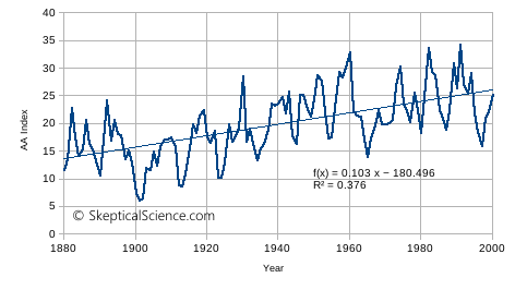
Figure 4. The AA index of surface geomagnetic activity.

We can break this down into the three components of the AA index, and graph them individually. This is done in figure 5.

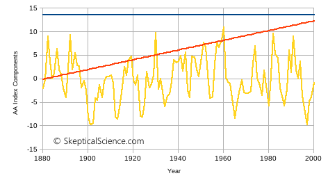
Figure 5. The AA index from figure 4, broken down into a constant value (blue line), a linear term (red line), and the remaining variation (yellow line).

What does this mean in terms of forcing the energy balance climate model? From figure 5, we see:

• The constant value component (blue line) implies that geomagnetic activity has a permanent forcing on climate. As long as there is any magnetic field at all, there will be a heat input into the earth-atmosphere system that will cause a continuous temperature rise.
• A linear increase over time. The heating effect of geomagnetic activity is getting stronger over the 20^th century.
• A variability (averaging zero) that follows the solar cycle.

This is inconsistent with the concept of radiative forcings. All the other forcings are expressed as a difference between normal equilibrium input and the current value - they are the energy that is pushing global temperature away from equilibrium. Remember that the Ziskin and Shaviv model assumes that emitted IR can be calculated based on ΔT, not T. If ISE starts with a large positive value in 1880, and rises from that point on, the model will find it very difficult to determine a reasonable value to use for the free parameter of ΔT at 0 radiative forcing.

The first component of the AA index makes no climatological sense. If it is permanent, what equilibrium is it upsetting? Why has the earth-atmosphere system not adjusted to this constant forcing?

• For all the known climate forcings, the “imbalance” term is usually specified by starting at zero at a specified time.
• In Ziskin and Shaviv, figure 2, we can see that their direct solar forcing (TSI) term starts at zero in 1880. So does the Aerosol indirect effect (AIE). Although they do not graph it, the greenhouse gas contribution will also be expressed as a change from normal – starting at zero, and changing over time.
• It is completely unreasonable for the ISE to begin at a non-zero value. If we use Ziskin and Shaviv’s most probable value of α_AA=2 (their figure 7), this constant component of ISE implies a forcing starting at 1 W/m² (2x the value in their figure 2) in 1880. This is a huge warming effect.

As far as I can tell, the only way for the Ziskin and Shaviv model to compensate for this constant input from ISE is to adjust the "ΔT at 0 radiative forcing" parameter and try to alter other free parameters to compensate.

The second and third components of the ISE – the linear trend, and variations – are more plausible. But do they really represent new information? Let’s look at the AA index compared to the TSI. Ziskin and Shaviv do not indicate which source they used for TSI data. I obtained several TSI reconstructions from http://www.leif.org/research/TSI%20(Reconstructions).xls, and chose the Wang values to compare to the AA index downloaded previously. Figure 6 graphs the two together. We see a high degree of similarity: both are increasing over time, and the variations show a high degree of synchronicity. The correlation coefficient between the two is 0.67 (r² = 0.45). This is not surprising. Geomagnetic activity is known to be affected by solar activity – but does it really give us additional information about how solar activity affects global temperatures?

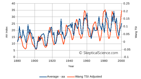
Figure 6. The AA index (yearly average, left axis) and the Wang TSI reconstruction (right axis). The axis scales were adjusted by eye to give approximately the same range.

Degeneracies and other model fitting issues

The problem with the high correlation between Ziskin and Shaviv’s use of TSI and ISE is that this causes problems in fitting these variables to their model. The TSI provides a direct estimate of radiative forcing for use in the model, but the ISE has to work through is fudge factor – α_AA. The TSI and ISE are both affected through the gain parameter – the free parameter that multiples the (1/λ)*ΔT term that counterbalances all terms in Ziskin and Shaviv’s ΔQ. How does the fitting process know whether to increase or decrease α_AA. or the gain, if it needs to enhance or reduce the overall solar effect to improve the fit?

The ISE also has issues with other forcings included by Ziskin and Shaviv, and I think that Ziskin and Shaviv know it. The paper mentions “degeneracy” seven times. What is a degeneracy? In this context, it is a difficulty in separating two terms that show very similar behaviour Which is the cause? Which is the effect? Are both terms caused by the same thing – i.e., they are not really independent? If I can multiply these inputs by any coefficient I want (“free parameter”), and I can make one bigger and the other smaller with little difference in the overall results, how can I tell I have a “good fit”?

Ziskin and Shaviv try to argue this is not a problem, but I am not convinced. In their closing discussion, Ziskin and Shaviv admit “...there is a large degeneracy between the TSI and the ISE. Namely, we cannot distinguish between hypersensitivity to the TSI (or some component of it), and an indirect effect, such as sensitivity to cosmic ray flux variations.” In other sections of the paper they state that there is a degeneracy between the positive effect of the greenhouse gas component and the negative aerosol indirect effect (AIE). They acknowledge that solar activity has a monotonic increase, similar to the monotonic increase in greenhouse gases and the monotonic decrease in the AIE.

They claim that there is no degeneracy between the TSI and other forcings, and the ISE and other forcings, but their argument (Section 4.2) appears to be little more than hand-waving. It amounts to “but oscillations” - the TSI and ISE have short-term variability that is not present in GHG or aerosol forcings, and this magically removes any co-dependence. We need remember, though: there three components of the ISE:

• A constant background forcing that causes continuous warming. This makes no sense climatologically, but surely will force the fitting procedure to minimize any other effects (probably by reducing the gain multiplier or changing the "temperature at zero radiative forcing"). There is a degeneracy here with all other forcings.
• An upward linear trend. This will cause degeneracies with GHG and aerosol forcings.
• Variability with a mean of zero. This will not be linked to linear trends in GHG or aerosol forcings, but their model also includes PDO and SOI terms. There is a strong potential that the ISE will have degeneracies with these terms, as well as with TSI variations.

Multiple degeneracies between the ISE and other forcings, on different time scales, does not seem like a convincing argument for “no degeneracies”. It seems that all the standard forcings are degenerate, but Ziskin and Shaviv’s preferred solar forcings stand out from the crowd. “I know you are, but what am I?” stopped being a good argument when I was still a child.

One last question to raise, before I run out of room. Well, one large question that is made up of several smaller questions.

• In section 4.3, Ziskin and Shaviv discuss adding the North Atlantic Oscillation (NAO), but explain how it did not improve the fit and causes issues with the ocean-land coupling.
• I cannot see any evidence that they tried to fit their model without their speculative ISE forcing.
• How well does their model fit if this term is not present? How much does the fit improve when it is included? They claim (section 5) that “the fit improves considerably if we include a solar forcing driver (ISE) other than the variations in the total solar irradiance (TSI)” - but where are the numbers?
• They do talk about optimal fits, and they give distributions of each fitting parameter to argue that ones with tight PDFs are better-determined.
• What are the actual values of each free parameter in their optimal fit?
• How much better is the fit when each of the different forcing terms area added?
• Statistical fitting can make use of concepts such as the Akaike information criterion (AIC) to evaluate whether adding addition parameters to a model improves the fit enough to justify the added complexity.
• Where is the analysis that shows the many free parameter terms in the Ziskin and Shaviv EBM actually improve the fit enough to justify their inclusion?
• Yes, by adding more parameters we can get the elephant to wiggle its trunk, but does this really paint a better picture of the elephant?

Conclusions

Overall, by including the ISE in their model,. Ziskin and Shaviv essentially force their model to do the following:

• Decrease the gain parameter, which essentially reduces the effect of all forcings. This fits the climate contrarian narratives of “greenhouse gases and aerosols are not that important” and “climate sensitivity is low”.
• Since decreasing the effect of solar activity is an undesirable outcome, adding a highly-correlated “indirect effect” allows for a magic multiplier on solar influence.
• Direct solar forcing (TSI) is small compared to direct GHG forcing, so if you want to argue that climate sensitivity is low (to argue against GHG forcing), direct solar influence sinks in the same boat (a smaller gain value in Ziskin and Shaviv’s model).
• By adding ISE, you have “special pleading” for solar. By having an extra multiplier (α_AA) that only affects ISE, you can make total solar effects much larger. “One of these things is not like the others. One of these things doesn’t belong.”

Throughout, Ziskin and Shaviv admit that they do not have a mechanism for their indirect solar effect, but claim they have found an effect anyway. This is a major weakness - “I don’t know what it is, but I know when I see it”. By using a geomagnetic index that creates an ever-present heating effect (the constant component of the ISE), they create an unreasonable physical climate model. By adding several non-radiative indices, each with its own fitting parameter, they create many possible degeneracies in model fitting.

Overall, I find the Ziskin and Shaviv paper extremely unconvincing. (Spoiler alert: there are no more spoilers.)

With a physically unrealistic ISE forcing, and so many free parameters to influence fitting their model, Ziskin and Shaviv not only fitted the elephant, they seem to have managed to get that elephant to paint their house “solar”.

Several common climate change myths relate to the discussion here, and are rebutted on Skeptical Science's list of popular myths:

#2 - It's the sun

#13 - Climate sensitivity is low

#21 - It's cosmic rays