Climate Science Glossary

Term Lookup

Enter a term in the search box to find its definition.

Settings

Use the controls in the far right panel to increase or decrease the number of terms automatically displayed (or to completely turn that feature off).

Term Lookup

Settings


All IPCC definitions taken from Climate Change 2007: The Physical Science Basis. Working Group I Contribution to the Fourth Assessment Report of the Intergovernmental Panel on Climate Change, Annex I, Glossary, pp. 941-954. Cambridge University Press.

Home Arguments Software Resources Comments The Consensus Project Translations About Support

Bluesky Facebook LinkedIn Mastodon MeWe

Twitter YouTube RSS Posts RSS Comments Email Subscribe


Climate's changed before
It's the sun
It's not bad
There is no consensus
It's cooling
Models are unreliable
Temp record is unreliable
Animals and plants can adapt
It hasn't warmed since 1998
Antarctica is gaining ice
View All Arguments...


Username
Password
New? Register here
Forgot your password?

Latest Posts

Archives

Radiative Balance, Feedback, and Runaway Warming

Posted on 26 February 2012 by Chris Colose

Skeptical Science has previously discussed the topic of feedbacks and why the existence of positive feedbacks (i.e., those feedbacks that amplify a forcing) do not necessarily lead to runaway warming, or even to an inherently "unstable" climate system.  I also wrote on it at RealClimate (and Pt. 2). This was brought up again in Lord Christopher Monckton's response to SkepticalScience, where he asserted:

"First, precisely because the climate has proven temperature-stable, we may legitimately infer that major amplifications or attenuations caused by feedbacks have simply not been occurring...A climate subject to the very strongly net-positive feedbacks imagined by the IPCC simply would not have remained as stable as it has."

I wanted to revisit the subject in order to take a different approach on the subject of positive feedbacks.  This involves the relationship between Earth's surface temperature and outgoing infrared radiation (the energy Earth emits to space). Determining how the outgoing longwave radiation (OLR) depends on surface temperature and greenhouse content is a fundamental determinant to any planetary climate.

I'll begin with very trivial, ideal cases, and then slightly build up in complexity in order to relate the problem to climate sensitivity.  By the end, it should be clear why positive feedbacks can exist that inflate climate sensitivity but do not necessarily call for a runaway warming case.  We'll also see a scenario, commonly discussed by planetary scientists, in which it does lead to a runaway.

First, we begin with the simplest case in which the Earth has no atmosphere and essentially acts as a perfect radiator. In this case, the outgoing radiation is given by the Stefan-Boltzmann equation OLR=σT4. T is temperature. σ is a constant, so the equation means that the outgoing radiation grows rapidly with temperature, (to the power of four) as shown below.
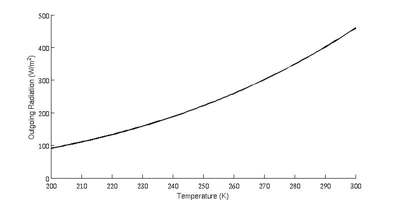
Figure 1: Plot of OLR vs. Surface temperature for a perfect blackbody


In the next case, suppose that we add some CO2 to the atmosphere (400 ppm).  The atmosphere here is completely dry (and therefore no water vapor feedback).  In this example, the addition of CO2 will reduce the OLR for any given temperature, since the atmosphere absorbs some of the exiting energy.  This is displayed with the red curve in Figure 2 (the black curve is from above for reference).
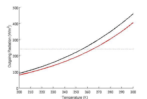
Figure 2: Relationship between OLR and surface temperature for a blackbody (black curve) and with 400 ppm CO2 (red curve).  The horizontal line is the absorbed solar radiation.

Also plotted in Figure 2 is a horizontal line at 240 W/m2, which corresponds to the amount of solar energy that Earth absorbs.  In equilibrium, the Earth receives as much solar energy as it does emit infrared radiation.  Therefore, in the above plot, the points at which the horizontal line intersect the black/red lines will correspond to the equilibrium climates in this model.  Note that the red line makes this intersection at a higher surface temperature, which is the greenhouse effect.

Now let's step up the complexity a bit.  We'll throw in some water vapor into the model, but not just a fixed amount of water vapor.  This time, we'll also let the water vapor concentration increase as temperature increases.  Water vapor is a good greenhouse gas, so now the infrared absorption grows with temperature. This is the water vapor feedback.  The blue line in the next  figure is the OLR for a planet with the same 400 ppm CO2, in addition to this operating feedback.
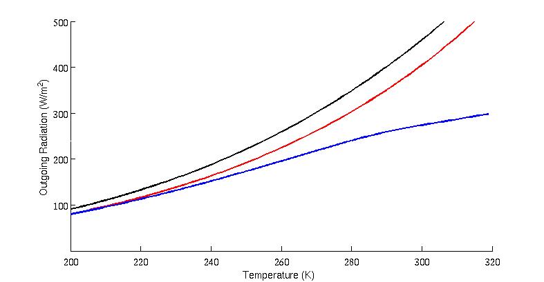
Figure 3: Relationship between OLR and surface temperature, as above, but with a constant relative humidity atmosphere (blue line, implying increasing water vapor with temperature)

In this figure, we see that the OLR does not depend very much on the water vapor at low temperatures.  This makes sense, because at temperatures this cold (such as during a snowball Earth), there is so little water vapor in the air.  However, at temperatures similar to the modern global mean and warmer, the OLR drops tremendously and the the T4 dependence instead becomes much flatter.  We'll get a more clear picture of that means for climate sensitivity in the next diagram.

In the next diagram, I've removed the red curve for convenience.  But I've added two horizontal lines this time.  You can think of this as two possible values for the incoming solar radiation. 
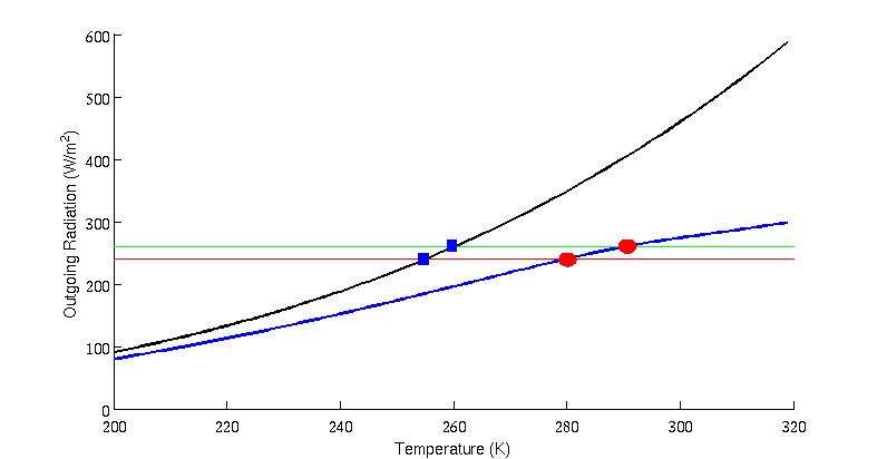
Figure 4: OLR vs. surface temperature for a blackbody (black curve) and an atmosphere with CO2 and a water vapor feedback (blue curve).  The horizontal lines give two values for the absorbed incoming solar radiation, and the colored shapes give possible equilibrium points.  On the trajectory where water vapor exists, sensitivity is enhanced because the temperature difference between the two red circles (as sunlight goes up) is greater than the difference between the two blue squares.

To interpret Figure 4, suppose that we increase the amount of sunlight that the Earth gets, which means we jump from the red to the green line in the above figure.  If the Earth were a blackbody (black curve) then the temperature change that results from this would just be the difference between the values at the two blue squares.  However, in a world with a water vapor feedback, the temperature difference is given by the distance between the two red circles.  We can infer from this that water vapor has increased climate sensitivity, yet it did not cause a runaway warming effect.

Now let's consider one more case.  Notice in the previous diagram that at very high temperatures, the OLR starts to flatten out, and indeed eventually can become almost flat.  This is due to the rapid increase in water vapor (and infrared absorption) as temperature goes up.  But suppose we pump up the amount of sunlight that the Earth gets to much higher values than in the last figure.  This new value is shown by the horizontal green line in the figure below.
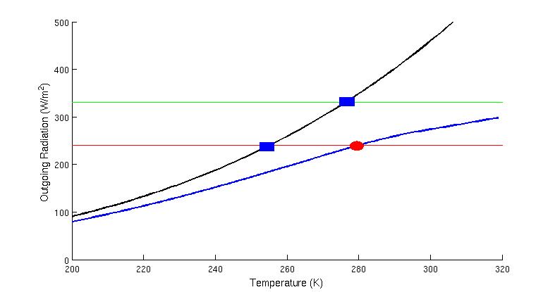
Figure 5: As above, but the green line corresponds to higher incoming solar radiation.

Once again, if we follow the black curve (with no atmosphere), then we get an expected increase in temperature as the amount of sunlight goes up.  But if we follow the blue curve (the system with an operating water vapor feedback), then something strange happens. 

At some point the OLR becomes so flat, that it can never increase enough to match the incoming sunlight.  In this case, it actually becomes impossible to establish a radiative equilibrium scenario, and the result is a runaway greenhouse.  This is the same phenomenon planetary scientists talk about in connection with the possible evolution of Venus or exoplanets outside our solar system.  The system will only be able to come back to radiative equilibrium once the rapid increase of water vapor mass with temperature ceases, which in extreme cases may not be until the whole ocean is evaporated.

From these figures, we can readily see the fallacy in "positive feedbacks imply instability" type arguments.  There is in fact a negative feedback that always tends to win out in the modern climate.  This is the increase in planetary radiation emitted to space as temperature goes up.  Positive longwave radiation feedbacks only weaken the efficiency at which that restoring effect operates.  Instead of the OLR depending on T4, it might depend on T3.9, or maybe even T3 at higher temperatures; eventually the OLR becomes independent of the surface temperature altogether.  I haven't discussed shortwave feedbacks, such as the decrease in albedo as sea ice retreats.  That only raises the position of the horizontal lines slightly, allowing for a warmer equilibrium point, but in no way compromises the argument.

In fact, the same sort of argument can be applied if we let the albedo vary with temperature (and so the absorbed solar radiation is no longer given by a horizontal line).  The opposite extreme, a snowball Earth, can then be thought of as a competition between the decreased longwave radiation to space as the planet cools, and the increased reflection as the planet brightens (when the ice line is advancing toward the equator).  As with a runaway greenhouse, it's not inevitable that this occurs, as is evident from times in Earth's history when ice advanced but did not reach the equator. 

As a final note, it's worth mentioning that it is virtually impossible to trigger a true runaway greenhouse in the modern day by any practical means, at least in the sense that planetary scientists use the word to describe the loss of any liquid water on a planet.  The most realistic fate for Earth entering a runaway is to wait a couple billion years for the sun to increase its brightness enough, such that Earth receives more sunlight than the aforementioned outgoing radiation limit that occurs in moist atmospheres.  None of this means that climate sensitivity cannot be relatively high however. 

Note: Except for the first graph, all computations here were done using the NCAR CCM radiation module embedded within the Python Interface for Ray Pierrehumbert's supplementary online material to the textbook "Principles of Planetary Climate."  The lapse rate feedback is included as an adjustment to the moist adiabat. I've assumed near-saturated conditions are maintained (constant 100% relative humidity) with temperature, although the argument is qualitatively similar with lesser RH values.

This post has been adapted into the Advanced rebuttal to "Positive feedback means runaway warming"

0 0

Printable Version  |  Link to this page

Comments

Prev  1  2  

Comments 51 to 98 out of 98:

  1. gallopingcamel, Just because there are thermodynamics equations in Nikolov & Zeller does not mean that they have been applied properly. N&K first argues that the usual simple radiative balance model (which by the way is valid for a rapidly rotating planet with large heat capacity) is bad, and then proceeds to apply an even worse model (i.e. one that is valid for a slowly rotating planet with low heat capacity) to argue that the greenhouse effect can't explain the large temperature difference; in reality this difference is mainly due to their model being wrong for a rapidly rotating planet like earth. Now in order to explain this large dubious difference between observed and their model, they proceed to invent a way to explain the difference. Their argument that temperature is driven by pressure is just pure non-sense. There is nothing in their argument that prevents me from arguing that temperature is driven by pressured. The ideal gas law does not tell you the causality. What they did manage to show with their data is that the ideal gas law holds very well for all planets with an atmosphere. Onto their main claim: The surface temperature is governed by nothing more than the solar irradiance and surface pressure (i.e. Ts=f(S0, Ps )). This analysis is fundamentally flawed. In the previous section they've demonstrated precisely that the ideal gas law is a good model for the atmosphere, which implies that there is a strong relationship between surface temperature and pressure. If they don't remove this effect, they are essentially asking how temperature depends on temperature itself, rendering their analysis moot. I have to check the above carefully, though my intuition tells me that this is not right) Even ignoring the above, they have eight data points, where two (mercury and the moon) is fitted automatically with the choice of function. They are left with 6 data points, and they have FOUR free parameters in their best fit. If this is not curve fitting, what is?
    0 0
  2. gallopingcamel, 3: So if you read point 2, you know that I am definitely open (based on my limited experience solving equations of the atmosphere) to the idea that the greenhouse effect may be neutered in general.. at least in the long run. However, all the planets and astral rocks considered (and I haven't read the main part of the article/paper yet, but have seen discussions related to observed patterns of natural pressure/temperature linkages in the atmosphere) have not been impacted by man. There is no direct evidence from other planets of what can or can't happen under a scenario just like the one we have on earth. These rocks in space don't have huge bodies of water, for example. And, they also don't support diverse lifeforms. Driving the planet beyond the natural range, at some point, can definitely lead to harm to (human beneficial) organisms (including humans) at a wide scale. In other words, we need something more quantifiable and germane to our current planet and the times scales key to our survival and well-being.
    0 0
  3. galloping- You are free to believe pseudoscience. I couldn't care less, nor does it have the slightest impact on the progress in scientific literature.
    0 0
  4. Looking at the "Unified Theory of Climate", I notice form equation (7), you have that: NTEPs = Ts/Tgb Substituting into equation (8), we obtain: Ts = 25.3966(S0 + 0.0001325) 0.25 * Ts/Tgb Dividing both sides by Ts/Tgb, we have (a) Tgb = Ts = 25.3966(S0 + 0.0001325) 0.25 Substituting from equation (2), we then have (b) 2/5 * {(S0 + 0.0001325) * (1 - Agb)/(es)}0.25 = 25.3966(S0 + 0.0001325) 0.25 where A stands for albedo (alpha), e stands for emissivity (epsilon), and s stands for the Stefan-Boltzmann constant (sigma). Hence we have: (c) [{(S0 + 0.0001325) * (1 - Agb)/(es)}0.25]/(S0 + 0.0001325) 0.25 = 63.4915 Cancelling out and distributing, we have (d) (1 - Agb)0.25/(e0.25*s0.25) = 63.4915 and hence (e) (1 - Agb)0.25/e0.25 =~= 0.8239 or, by raising both sides to the fourth power: (f) (1-Agb)/e =~= 0.4607 We are told that (g) Agb =~= 0.125, and hence (h) 1/e =~= 0.5265 or (i) emissivity approximately equals 1.9 which is impossible. OK, maths is not my strong suite, so it is entirely possible I have made an algebraic error above. If so, could somebody please point it out to me. But if not, why are we paying attention to this ridiculous theory which can be true only of the laws of thermodynamics are false.
    0 0
  5. Tom Curtis, I think the problem is at step b because eqn 2 forms part of a criticism of the 1 shell model, and I don't think it goes with section 3, where a new theory is covered. @IanC >> Their argument that temperature is driven by pressure is just pure non-sense. There is nothing in their argument that prevents me from arguing that temperature is driven by pressured. I think you meant that we could argue the converse, that pressure is driven by temperature. What do we know about restraints on volume (or concentration of particles)? I had seen a wikipedia reference (that I can't find this second) relating adiabatic polynomial adiabatic 7/2 power to degrees of freedom polynomial 5/2 power to predict some natural balance in volume increases ... ???
    0 0
  6. Chris Colose, if there is some value to the idea that pressure of the atmosphere (assuming it has some amount of ghg) is intimately linked to lapse rate and temperature, observations on earth at our human life timescale do appear to show strong correlations between unpredictable and human changes to the atmosphere and results in temperature. These drivers cannot be called natural cycles. In fact, even natural cycles, as long as they are not driven by the sun, would appear to contradict any such theories. There at least would be a strong argument that the best descriptions of short-term changes have been captured in climate models. A steady state over millions of years perhaps is immaterial to the main question over our fate.
    0 0
  7. Jose_X @55, I see what you are saying, but equation (7), which is definitely part of the new theory explicitly includes the therm Tgb. What is more, their figure 5 plots the ratio of Ts to Tgb. Hence Tgb is definitely part of the new theory. The only definition they provide for it, however, is in equation (2) and related discussion. Therefore, that is not a flaw in my algebra. It is at best a flaw in their presentation, such that they do not have a theory until they provide us with an alternative definition of Tgb, assuming, of course, no other error in my algebra.
    0 0
  8. Tgb is not part of the one layer model, it's just a new definition of the gray body temperature. It assumes a temperature distribution proportional to the cosine of latitude to the 1/4 which gives a temperature at the poles of zero Kelvin and of about 360 K at the equator (for the Earth). This makes sense in the no-atmosphere, local equilibrium, case like the Moon. Given this definition, though, Tgb can not be compared to the effective radiating temperature to quantify the greenhouse effect.
    0 0
  9. Riccardo @58, it partially makes sense for a no-atmosphere, local equilibrium case. As calculated, Tgb assumes no thermal inertia, and no thermal distritution through conduction (or any other means). That is as unrealistic an ideal case as the standard "effective temperature", which in effect assumes absorptivity of 1, and perfect heat distribution so that no point on the surface has a different temperature than any other point. The practical importance of the effective temperature is that it is a maximum mean surface temperature that can be achieved without a green house effect. Conversely, Tgb calculates a theoretical minimum temperature for a body without an atmosphere. As such it is very surprising that Nikolov and Zeller report an observed mean surface temperature for the moon equal to their calculated mean surface temperature, ie, 154.3 K (table 1). Pressed to justify this figure on WUWT, Nikolov justifies the value by appeal to Vasavada et al, 1999 who report modelled mean lunar surface temperatures of 220 K at the equator (figure 3), and 130 K at 85 degrees north (figure 4) (also reported by wikipedia). Calculating the mean as (140 plus 140 plus 220)/3, yields a mean surface temperature of 167 K, which is probably an underestimate. Nikolov also appeals to Diviner, which reports a mean equatorial temperature of 206 K, and a mean polar temperature of 98 K (mean of equator plus two poles: 134 K, but the averaging method leaves much to be desired) Nikolov himself calculates the mean form the diviner data as (100+206)/2 or 153 K. These very low values contradict the subsurface measurements at the Apollo 15 (26 degrees North) and Apollo 17 (20 degrees North) sites. They show a subsurface temperatures approaching 253 K (Apollo 15) and 257 K (Apollo 17) conservatively estimated, showing these temperatures to be the mean surface temperature for those sites, ie, in a sub-equatorial region the mean temperature is at least 30 degrees K higher than estimated by the model, and nearly 50 K higher than estimated by Diviner. Consistent with that, Daniel Harris cites Peter Eckart ("The Lunar Base Handbook", 2nd Ed 2006) to the effect that the polar region (excluding shaded craters) has a mean of 220 K, while equatorial regions have a mean of 255K. (Rough estimate of the combined mean: 230 K). I have also seen figures of 243 K and 250 K cited with dubious provenance. I have been unable to find relevant figures from the Chang E-1 satellite The important thing about this is that while Nikolov and Zeller report an observed mean surface temperature of the moon as being 154.3 degrees C, clearly the observation made in determining that value was that that was what their theory predicted. In some circles reporting theoretical predictions as being observed results is frowned upon. That Nikolov and Zeller are prepared to do so, however, calls into question the remarkable "predictive accuracy" of their theory as shown in their figure 5. It may well be that for many values, and not just for the Moon, what is "accurately predicted" is just the value calculated in the prediction.
    0 0
  10. Jose_X 56, Yes of course, I meant pressure driven by temperature. Thanks for pointing out the mistake. (Mods: is there a way to fix the error in my post in 51?) Can you elaborate your question? Are you talking about the substance in gas phase? or in solid or liquid phase? Tom Curtis 57, I think you made a mistake after step (d). For (e) i got 0.9797, and from here I have (f) (1-A)/e = 0.912 (g) A=0.125 (h) 1/e=1.0423 ==> e= 0.9594
    0 0
  11. IanC @60, you are correct. Thankyou for taking the trouble of checking.
    0 0
  12. Reading Nikolov and Zeller's second article on WUWT cracks me up. They kept on insisting that their answer must the right one, so if the observation differs from their answer they should just use their calculated answer to as the observation. The real gem is the following:
    In a recent analytical study, Smith (2008) argued that Eq. (5) [refers to N&K's grey body model] only describes the mean temperature of a non-rotating planet and that, if axial rotation and thermal capacity of the surface are explicitly accounted for, the average temperature of an airless planet would approach the effective emission temperature. It is beyond the scope of the current article to mathematically prove the fallacy of this argument. However, we will point out that increasing the mean equilibrium temperature of a physical body always requires a net input of extra energy. Adding axial rotation to a stationary planet residing in a vacuum, where there is no friction with the external environment does not provide any additional heat energy to the planet surface. Faster rotation and/or higher thermal inertia of the ground would only facilitate a more efficient spatial distribution of the absorbed solar energy, thus increasing the uniformity of the resulting temperature field across the planet surface, but could not affect the average surface temperature. Hence, Eq. (6) correctly describe (within the assumption of albedo uniformity) the global mean temperature of any airless planet, be it rotating or non-rotating.
    Again, they would just assert that their model is correct. They are unable to mathematically prove Smith 2008 to be wrong because Smith 2008 is correct: rotation and heat capacity do matter, and N&K's solution is merely a special limit, obtained by taking rotation speed to infinity or heat capacity to zero. It is particularly ironic because N&K repeatedly invoked Holder's inequality, and argue that one must be careful when integrating a non-linear quantity. If they really were this careful, they would realize that calculating the average surface temperature of a spherical object is inherently non-linear, so increasing the uniformity of temperature will certainly change the answer. I know that Smith2008 has been mentioned here on SkS in a post on Postma, but are there plans for a detailed explanation of the Smith 2008? Also, given that N&K's theory is starting to appear, is there a rebuttal planned?
    0 0
  13. Tom Curtis #57, I see IanC spotted a mistake, and I have not read the whole article; however, this remark they made would make me very suspicious that they would decide to use this Tgb value: > Since in accordance with Hölder’s inequality Tgb ≪ Te (Tgb =154.3K ), GHE becomes much larger than presently estimated. > According to Eq. (2), our atmosphere boosts Earth’s surface temperature not by 18K—33K as currently assumed, but by 133K! This raises the question: Can a handful of trace gases which amount to less than 0.5% of atmospheric mass trap enough radiant heat to cause such a huge thermal enhancement at the surface? Thermodynamics tells us that this not possible. We know that this Tgb is very low compared to observations of T, so I take this as a rejection of the modified 1 shell model rather than as a way for the authors to introduce a model that they believe does justify 133K. I'll try to finish reading soon. @Everyone: I wanted to ask people here what they think about this: http://theendofthemystery.blogspot.com/2010/11/venus-no-greenhouse-effect.html . Skimming should give an idea of the main claim. A summary might be that the top section of Venus' atmosphere (50km altitude and up, where the pressures exist on Earth) matches the Earth's atmosphere in temperature once we factor in the ratio of the Stefan Boltzmann calculation for Venus to that of Earth (ignoring albedo!). Although I have been critical of it without passing an official final judgement (note how Venus has similar mass, radius, and hence gravitational constant as Earth), it seems to cast some doubt to what all of that CO2 is doing. Note, the albedo is entirely ignored by Huffman (and this appears to present conservation of energy issues or information traveling faster than speed of light so that emitter A can generate extra radiation beyond S-B to match what B will reflect, etc.. but maybe not (I won't detail guesses I have)). Note that the values used for Venus might be a little off. I found what looked like an authoritative source (need to hunt down the link). While the numbers are a little off from what I saw, they are in the right ballpark (but the deviation is a bit greater). I can imagine that the lapse rate changes shape deeper into Venus, but I think data suggests it is close to a line of similar slope to that of the earth (?). It's also true that right below the top 1 atm isn't a body of water and earth but instead just more air so it is not the same scenario as Earth. A question that follows would be, if the atmosphere was largely N2, would this same general lapse rate exist down to the ground, possibly with only a little bit different slope? Also, would the slope be significantly different or would the rate be a different very distinct curve? Anyway, my main problem is that I don't yet know clearly the equations/algorithm that predict GHE (eg, Ramanathan and Coakley '78), so I can't carry out a few quick checks. If all there was to average temperature was the pressure, we would not experience large oscillations. I don't know what level of variation (eg, deviations from solar tracking.. as CO2 on earth is predicted to be causing for decades now) would be consistent with such a view. There is too much data I have not seen/analyzed and too much theory I still haven't covered. Obviously, I can consider that maybe there are some mistakes in our current understanding of GHE. Or, I can consider that a strong GHE effect leads to 1%-10% or other maximum variations near the surface (a limit I did not think existed). This would bound the earth temperature above (against GHE predictions I think), if still allowing great threat to humans. Anyway, I assumed the WUWT paper being discussed was related to what the Huffman webpage shows. Assuming it is, I don't worry too much about astral rocks with light atmospheres (our high altitude low pressure atmosphere deviates from the lapse rate), but moon Titan might be another example following the Earth/Venus ratio. Any opinions?
    0 0
  14. Tom Curtis #57: I think I understand where Tgb comes from. The part inside the integral of eqn 2 (which looks like eqn 1 without the 4 denominator) is just Stefan-Boltzmann in a form that shows the value of T explicitly as a function of power flux. This starting point is independent of the shell radiative model, and numerous people accept it and use it to calculate the temp of the planet if it had not atmosphere. The albedo would be to sun's radiation and the emissivity would be for the planet radiating in its own spectrum range as graybody. This is consistent with how it refers to Tgb later on, "the average temperature of a Standard Planetary Gray Body (SPGB) with no atmosphere (Tgb, K)." And then it clarifies that it is using that Tgb with reasonable parameter values: > We employ Eq. (2) to estimate Tgb assuming an albedo αgb = 0.12 and a surface emissivity ϵ = 0.955 for the SPGB based on data for Moon, Mercury, and the Earth surface. Using So = 1362 W m-2 (Kopp & Lean 2011) in Eq. (2) yields Tgb = 154.3K and NTE = 287.6/154.3 = 1.863 for Earth. This prompts the question: What mechanism enables our atmosphere to boost the planet surface temperature some 86% above that of a SPGB? I agree then that step b is correct.
    0 0
  15. I understand that it might be just my prejudice but I'm not sure I want to read something (as Jose_X suggests) written by someone introduced by these words, they doesn't sound much like well founded science:
    "Science today recognizes the world was remade (through a presumably long process of continental breakup, worldwide drift, and rejoining), incredible as that seemed a hundred years ago. "The End of the Mystery" establishes the even more astounding, and even surer, fact that the world was deliberately changed, to enable a great design. It is only the overwhelming scale of the design that has up to now stymied man's understanding, eluding even the finest modern scientific minds. The discovery of a great, world-encompassing design, confirmed alike by new, overwhelming physical facts about the Earth and by the universal ancient testimony, invalidates the presumption against design of the current scientific consensus, and enlightens both religion and science. We are in fact at the start of a new age of unprecedented, unified understanding, of the real history of the Earth and man.
    For what is worth, I don't understand why Jose_X keeps quoting pages of "strange" science while leaving the door open to the possibility they're at least in part correct and that "it seems to cast some doubt to what all of that CO2 is doing."
    0 0
  16. Ricardo, (-snip I was going to state at the top of that comment that here was a person who had been [pick horrible deed X done to a child] by a climate scientist.-) I summarized the results. I am curious what you think about what I wrote. If you want more details, ask or glance at that page I linked. My problem essentially is that I don't have a handy solver to test out what the GHE calculates for the surface temperature of Venus. Next (problem 2), replace most of that CO2 by N2 and see what is the result. Can you help me with these two calculations to see if the first one fits the data and then to see (out of curiosity) what the second one produces?
    0 0
    Response:

    [DB] Inflammatory snipped.

  17. Jose_X you have three possibilities, look at what other scientists published on the topic or read a textbook on radiative transfer and do proper calculations yourself or satisfy your curiosity with a crude semi-quantitative model. The latter is straightforward. If you have a transparent atmosphere you end up with a isothermal atmosphere at the same temperature as the surface; the latter is determined by simply balancing the fluxes. In the real case, use the adiabatic lapse rate, the emission altitude from the effective radiation temperature and extrapolate back to the surface. But please, stop quoting from bad science sites ...
    0 0
  18. Jose_X at 16:41 PM on 29 February, 2012, You have identified the main weakness in the references I cited. They lack a physical mechanism to underpin them and that leaves them open to the charge of "curve fitting". Remember that Alfred Wegener had been dead for many years when the scientific world stopped laughing at his theory of "Continental Drift". Nicola Scafetta is all too well aware that even if his prediction of global temperatures to 2040 proves to be more accurate than that of the IPCC's AR4, it proves nothing unless he can explain the underlying processes. He is making progress and I find his ideas quite plausible. When he "goes public" we will be able to take this discussion to the next level. In my opinion, N&K are in the same boat but I have not had the opportunity to meet them. (-snipIn AR4, the IPCC used a composite of a portfolio of models that are also open to the charge of "curve fitting". Richard Lindzen included a table of the parameters used in these models in his recent address to the UK House of Commons. This was a dubious approach in AR4 and according to Alec Rawls it will be even more dubious in AR5. http://wattsupwiththat.com/2012/02/22/omitted-variable-fraud-vast-evidence-for-solar-climate-driver-rates-one-oblique-sentence-in-ar5/-) Early drafts of the AR5 Working Group 1 have been leaked and I have a team working on them. You are clearly a deep thinker so would you be interested in participating? http://www.gallopingcamel.info/IPCC.htm
    0 0
    Response:

    [DB] Imputations of impropriety and fraud snipped.  Please pay more than a passing nod to the Comments Policy of this site.

  19. The majority of this comment (middle on down) serves to illustrate a misunderstanding that perhaps a number of people might be having. >> please, stop quoting from bad science sites Riccardo, I brought up a point that presumably is based on data and which is a reasonable question to ask of the GHE since on the surface appears to suggest the amount of ghg does not matter. I linked the webpage for reference to reduce the number of replies asking for more detail. >> If you have a transparent atmosphere you end up with a isothermal atmosphere at the same temperature as the surface My second scenario is not 100% N2 (which is this simple case you answered). Essentially, I have not verified that there is an appreciable difference between having a small amount of CO2 vs having almost the entire atmosphere be CO2. In Venus, we have a number of similarities to the Earth but the opposite extreme as here in terms of relative proportion of ghg. Has no one published a paper applying GHE equations to Venus? [See conclusion below, as it suggests a classroom exercise might be more appropriate.] >> In the real case, use the adiabatic lapse rate, the emission altitude from the effective radiation temperature and extrapolate back to the surface. This approach was exactly what gave me a little concern. I think it's also what Joel Shore describes in part (c) of his reply here http://wattsupwiththat.com/2011/12/29/unified-theory-of-climate/#comment-849734 Let me take this slowly. If we initially only concern ourselves with a rough approximation, then the webpage I linked takes you through the data to suggest that we would get exactly the same answer regardless of the amount of CO2. The slope of that lapse rate appears to be about the same for Venus as for Earth.. again, to first approximation. Now, I would not have expected this result.. even to first approximation. Now, on to more precise estimate considerations. One of my next thoughts was that the lapse rate is basically linear over a narrow pressure range (or more linear nearer to TOA?) but then bends on the way down in very high pressures. This would perhaps solve the problem. As we go deeper into Venus, the curve would bend towards higher temperatures.. in comparison to the path it would take if Venus has the % makeup as the Earth has. [Update to self: the graph here http://en.wikipedia.org/wiki/Atmosphere_of_Venus#Troposphere appears to show a slight bend towards higher temperatures in the low part of the line] This is why I ask about a precise calculation. Now, let's look at a few potential curves more closely. First, I have the question of what to expect, so let's consider some possibly hypotheses. H1: I know that 100% CO2 perhaps might not make much of a difference vs 10% CO2 + N2. I don't know but some degree of saturation certainly could be in play. H2: In fact, the actual physics could potentially make the 100% CO2 case do worse. These are all possibilities a priori. H3: A different form of reasoning might hypothesize that more CO2 should *always* lead to greater GHE within the limits imposed that a doubling of concentration leads to linear temperature increases. This is the standard model, I think, so I will look at it first. I now look towards the Earth predictions. We have a few degrees.. or let's say 1 K for 2xCO2. Extending this, 1 million xCO2 (approx 20 doublings) would lead to 20 K increase. 20K increase!! OK, maybe the model is being driven out of range by my example of 1 million fold increase. This would lead to about 390 atmospheres of pressure at the surface of the Earth and near 99.99% CO2. Or maybe the model would hold. Very interesting result. I did not expect that. I'll stop here since it appears I might have my answer from standard theory. My conclusion is that the climate models would appear to be consistent with the Venus example since a small change in slope is enough to change the temperature at the surface of Venus by about 20 K (or vicinity) rather easily. My concerns have been dispelled for the most part (pending a recheck of the logic and math). After thought: On earth we can have a very modest change in pressure of 40% via 1000 fold increase in CO2 yet get a full 10K. This 10K would be more than half of the 18K or so ballpark figure representing the super hot and high pressure Venus. This result is certainly a bit counter-intuitive (thanks to the log relationship).
    0 0
    Moderator Response: [JH] Please refrain from using this comment thread as your personal scratch pad.
  20. I think I resolved my Venus/Earth conflict http://www.skepticalscience.com/news.php?p=2&t=53&&n=1310#75971 . Believe it or not, that particular planet comparison had been nagging me for at least a few weeks. None of my few replies addressing it (on a different forum) had simply calculated the 10^6-fold increase scenario to make it apparent that there was no inconsistency between that data and GHE.
    0 0
  21. "Remember that Alfred Wegener had been dead for many years when the scientific world stopped laughing at his theory of "Continental Drift"." So who stopped laughing? The idea that continents could move over the seafloor was and still is ridiculous. His observational evidence that eventually helped lead to modern tectonics was not ridiculous and not laughed at. However, where are the unexplained puzzles in climate theory comparable to Wegener?
    0 0
  22. Moderator JH from #69, I thought I asked a reasonable question about radiative balance. If I kept quiet about the resolution, the question stays on the comment thread unanswered. Was that the preferable option? Is it my fault I didn't know the answer when I asked it and later realized it? Is there no use to detailing an answer? Is it not useful to present the sort of honest thought process that goes through people's minds? I thought this thought process (the form of #69) is useful to a website trying to understand its audience so as to better communicate the website's message. I'm not the best writer. Was that the problem?
    0 0
    Moderator Response: [JH] Suggest that you do your calculations off-line and keep your comments focused. People are just not inclined to read lengthy rambling posts.
  23. scaddenp @71, Scafetta has shown that planetary motions correlate with global temperature. At first blush this sounds like astrology rather than science. You should be skeptical as I am but maybe we should suspend judgment. Suppose that the gyrations of the major planets somehow modulate the reactions taking place in the sun's core. If this was happening, how long would it take for the effects to reach the sun's radiating surface? If you rely on Radiative Transfer the answer is tens of thousands of years. So is there any process that could explain the very short time constant that matches observations? If such a mechanism exists it may take decades to understand it just as in Wegener's case.
    0 0
  24. Jose_X - I will (putting my 2 cents in, if that) note that it is a bit difficult to follow a stream of consciousness post. It would be easier to follow if you were to note your assertion(s), followed by the backing. Otherwise it's a bit difficult to identify any issues you might raise. That said - Huffman appears to think that plate tectonics is nonsense (not the best recommendation), N&Z have apparently used basic curve fitting to re-derive the S-B relationship without acknowledging it, PV=nRT requires a separate temperature driven by convection and radiative physics to set the pressures, etc. Even WUWT has pointed out N&Z issues with significant justification. Which aspect(s) of those postings do you consider significant issues with basic radiative physics?
    0 0
  25. gallopingcamel - Scafetta's work is simply curve-fitting to a limited period. When taken outside the 'training period' for his cyclic+quadratic fit, it fails horribly: This is simply a rather limited Fourier decomposition (over-attributed to larger frequencies within the timeframe that happen to somewhat match selected astronomical periods) of the period under analysis, with no predictive power whatsoever - correlation without causation, unable to make any predictions as it is not based upon any physics related to the system. That's fine as long as the inputs/forcings do not change, but cannot predict future (or past, as shown above) behavior if they do, for example as CO2 levels change. I'll note that the quadratic term in Scafetta's most recent work (oddly without emphasis in his papers) does roughly correspond to CO2 forcing. With no conclusions drawn, or analysis applied... Where is your skepticism?
    0 0
  26. My apologies, the Loehle/Scafetta reconstruction in the illustration has a cyclic+linear component. The most recent Scafetta paper, on the other hand, has a cyclic+quadratic basis up until ~2000, when (for reasons not clearly justified, or understood here, as it leads to a worse fit) he changes to cyclic+linear again. Either way, his model fails in backprojection, includes no physics, but is simply correlation without causation, and hence has no predictive power. Physics: Good predictions Good stats: Reasonable predictions if nothing changes Bad stats: Better off repeatedly flipping a coin Since CO2 forcings are constantly changing, ENSO, solar, and volcanic forcings are not correlated, Scafetta's work is simply bad statistics.
    0 0
  27. Jose_X @70, Your calculation based on CO2 doublings greatly underestimates the effect of multiplying Earth's ~400 ppm of CO2 by a factor of one million. Adding that much mass to our atmosphere would raise the surface temperature to at least 900 Kelvin. Once the surface temperature gets high enough the oceans would vaporize causing an additional 300 bars of surface pressure and a further increase in temperature. Venus with its 90 bar atmosphere would look chilly by comparison. Chris Colose would (posthumously) call this a "Runaway" greenhouse effect. You can find an excellent discussion of this here with plenty of side references that are worth reading: http://scienceofdoom.com/2010/06/12/venusian-mysteries/
    0 0
  28. KR @74, 75 & 76, As acknowledged in my #68, Scafetta's model is open to the charge of curve fitting as are all the IPCC models. Scafetta understands that the "hard part" is to develop a theory to explain why his model is more than just curve fitting. See my #73. The IPCC models suffer from confirmation bias because they assume that CO2 is responsible for most of the recent warming while ignoring the evidence that 50-80% is attributable to natural causes.
    0 0
    Response:

    [DB] "The IPCC models suffer from confirmation bias because they assume that CO2 is responsible for most of the recent warming while ignoring the evidence that 50-80% is attributable to natural causes."

    Unsupported assertion.  It is incumbent upon you to now provide links to peer-reviewed articles published in reputable journals that document that the evidence you mentions both exists and that the IPCC has ignored it. 

    You will be held accountable for the above statement.

  29. galopingcamel "they assume that CO2 is responsible for most of the recent warming" I'm sure you know this isn't true.
    0 0
  30. I didn't expect to have 2 people look up Huffman. Were he the true Mickey Mouse, I'd still want an answer to the pattern. I did think the Venus/Earth pressure-temp example was most likely not new (although maybe it was based on very new astronomical data). KR #75 #76 >> Since CO2 forcings are constantly changing, ENSO, solar, and volcanic forcings are not correlated, Scafetta's work is simply bad statistics. From the limited amount I read and keeping in mind I don't know the state of climate science, I think I came across one positive point but maybe more. The analysis may have identified or refined the understanding of known global cycles. Recognized local cycles (PDO, etc) along with anything else can lead to global cycles not yet studied (for example, identifying resonant planetary frequencies). As evidence that the analysis might be statistically significant, the paper split the 1850-2000 time period into 2 pieces and then showed that tuning to either piece did a reasonable job "predicting" the other. This suggests that over a period of 50-100 years, incorporating cycles tuned from past data may improve the accuracy of one or more existing climate models. [I'd be curious to know how sensitive were the results to the split point date.] The CO2 trends are effectively a conditional prediction (along the lines of IPCC scenarios) that form a necessary part of the procedure. I agree with your comments on the paper otherwise: on the value of physics, on the unsupported conclusions/projections, and on the probable lack of significance of the astrological cycles (although I agree with gallopingcamel that further physics-based analysis might yield fruits). >> When taken outside the 'training period' for his cyclic+quadratic fit, it fails horribly To be fair, models come with limits by definition (although it might be a useless model for making predictions). The main failure has to do with no reasonable guesstimate for a trend curve going far back. This failure is independent of frequency analysis. To illustrate this point of model limits, if we halve CO2 levels in Earth atmosphere just 30 times, the logarithmic predictions used by at least some useful climate models will be wrong since this would result in a temperature noticeably below the simple S-B result for Earth+atmosphere (also calculating some extra loss of temp from H2O vapor reduction and even considering aerosols), incorrectly implying the GHE of remaining amounts of ghg is negative. gallopingcamel #77 Yes, the Earth case would be worse because of H2O and maybe a significant amount of methane and/or something else. For understanding the Venus data and to challenge GHE, I chose to limit to CO2 and generally be on the conservative side.
    0 0
  31. >> For understanding the Venus data and to challenge GHE, I chose to limit to CO2 and generally be on the conservative side. Scrap! I through I had this right. No, actually the "conservative" 1 K step I used makes it easier (not harder) to find agreement with GHE. If I really wanted to test GHE, I would have gone with a larger number. Anyway, the concept was demonstrated: that doubling a trace ghg gives a high bang for buck in terms of warming, while doubling an abundant ghg doesn't do so much extra vs doubling an abundant non-ghg.
    0 0
  32. Jose_X - "The main failure has to do with no reasonable guesstimate for a trend curve going far back. This failure is independent of frequency analysis." I would greatly disagree. There are now about a dozen decent proxy reconstructions of temperature for the last thousand years or so - with no major disagreements. As shown in the comparison here, Scafetta's cycles diverge drastically outside their training interval. They fail in hindcasting, which provides zero evidence that they will succeed in forecasting. Frequency analysis can be helpful in attribution and identification of causal relationships - but it cannot stand alone. You need to follow up by examining the physics. Scafetta performed a very basic frequency analysis on a certain period of one temperature record (not crosschecking against more than one temperature record, incidentally), made some very odd data processing choices (there's a frequency peak at ~4 years, which he does not discuss - but he runs the temperature data through a 4-year smoothing, which eliminates it!), and then fits those frequencies to various astronomic periods without a causal link. That's about as straightforward a case of Correlation without Causation as it gets. Going on the physics, on the other hand (as in Lean and Rind 2008, and in Foster and Rahmstorf 2011), including radiative physics: start with a causal link, examine the time evolution of the forcings for attribution, and from that determine the influence and weighting of various inputs - that has both hindcast and forecast capabilities. And, given that said attributions do account for the evolution of the temperature record given our knowledge of the forcings (within quite small variations), Occam's Razor indicates that invoking mysterious cyclic influences via unsupported linkages is both unnecessary and foolish.
    0 0
  33. My apologies, my previous comment should have been redirected to the Scafetta Widget thread to stay on topic. Please respond re: Scafetta there.
    0 0
  34. KR, we might be miscommunicating a little, but I'm sure we are also disagreeing. 1: I accepted the hindcasting was horrible before 1850. My comment was that no attempt was made to find a "trend line" going back beyond 1850. The model states essentially 1850 0 0
  • The browser didn't show me #83 until after submitting #84 (in rep to #82).
    0 0
  • It seems the webserver garbled the < I had used in comment #84. I'll repeat a large paragraph near the top: I accepted the hindcasting was horrible before 1850. My comment was that no attempt was made to find a "trend line" going back beyond 1850. The model states essentially 1850 < t < 2000 and 2000 < t < 2100 iirc. To hindcast further is interesting but void. The trends are clearly very important to approaching the actual temperature values and were not done. Reusing the linear trend (or had you used the linear and quadratic) as you do is interesting but void. The true older trends likely represent very long term cycles or no real "cycles" at all. [If the analysis were to be extended further, you would probably want to use a large basis set (sinusoids and maybe even polynomials, wavelets, etc) and not just two "trend" curves.] Anyway, without the longer analysis, the short-cycle analysis doesn't become void, but, yes, further back hindcasting will almost surely fail. Now, the short-cycle ....
    0 0
  • Can the Scafetta comments (#82-#86 and this one) be moved over with a link back to this thread for reference purposes? I really wasn't interested in analyzing that topic here (or now) and apparently neither is KR. FWIW, I like the gist of this comment http://www.skepticalscience.com/news.php?n=1293#75633 and found KR's http://www.skepticalscience.com/news.php?n=1293#75634 informative.
    0 0
  • Jose_X - I have replied here.
    0 0
  • I noticed a piece at the beginning of #66 was snipped. "Ricardo, (-snip-)". It's probably a good thing that was snipped although no insult was intended. Here is a translation of what I had written. "Ricardo, I was going to state at the top of that comment that Huffman appears to have a lot of anger towards the climate science community." The intention of that line above would have been to warn anyone who went to read that link not to get distracted with the snide remarks (and outright insults) against climate science that pepper the website; however, I did opt not to forewarn anyone when I provided the link, and then Ricardo apparently found the link offensive and made it clear he did not like/trust the person. Of course, I was not asking anyone to like or trust the person. As I already explained, I had offered the link for reference purposes to the question I had about the GHE on Venus.
    0 0
  • Ricardo 67>> In the real case, use the adiabatic lapse rate, the emission altitude from the effective radiation temperature and extrapolate back to the surface. I do thank you for the advice even though in this case I already knew what you stated, but the problem is that if we are going to test GHE vs no such effect I don't think measuring the lapse rate is acceptable since we only have one Venus like planet to measure (so we can't measure the w/GHE and also the w/o GHE cases). The idea would be to derive the lapse rate for the GHE and for the non-GHE cases and compare those two to each other (and while we are at it, compare the GHE case to Venus measurements).
    0 0
  • Jose_X we already talked about the no-GHE case and you replied that it was not your interest ("My second scenario is not 100% N2 (which is this simple case you answered)"). Keeping in mind that we're talking about a rather crude aproximation, if you have a not too low absorbtion the lapse rate is not determined by the exact amount of greenhouse gas absorption, it's determined by specific heat and gravity. Where absorption matters is in the optical thickness as function of height needed to determine where to start extrapolating backward to the surface. You may easily understand that it's not by chance or other weird reasons that the temperatures in Venus and Earth atmospheres are similar for equivalent pressure levels. It's not that "it seems to cast some doubt to what all of that CO2 is doing."
    0 0
  • GC - why would you give time to such astrology when there is perfectly good physical explanation for climate? Scafetta has another problem - how to explain why the known physical properties of GHGs do NOT affect climate, given the observed effects on DLR.
    0 0
  • Ricardo, currently a moderator (JH) believes I am "meandering". I asked for clearer guidelines on what to comment and what not to comment, eg, so I can avoid this "meandering". http://www.skepticalscience.com/news.php?n=1293#76064 I did not major in communications, that's for sure. And it does bother me not to come through clearly. To keep this fairly short, thanks for your information (the optical thickness part). I still think there is an apparent coincidence not yet covered on the temperature-pressure near matchup. [I would have to calculate optical thickness height to the lower .7 albedo flux at TOA and verify that this Venus lapse rate line sort of overlaps the similar slope line on earth by the time the pressures line up.] And the "non-GHE" case was not of 100% N2 with absolutely no ghg (I should have been clearer) but of using very low ghg % such as we find on earth. The 0 GHE case is trivial, as you pointed out. Sorry for the confusion.
    0 0
  • @ Jose_X #68 I try to give some answers. 1) Atmosphere 100%N2 The atmosphere is perfectly transparent and so isothermal: that’s, Ts = Tt = Tef where ‘s’ is surface, ‘t’ is TOA and ‘ef’ is effective. 2)Let’s add CO2 as 300 ppm as for Earth The balance of radiative power is (missing the constants) xTt^4 + (1-x)Ts^4 = Tef^4 Tt/Ts = (Pt/Ps)^(R/Cp) Ht = (Ts-Tt)Cp/g where ‘x’ is the % of radiation in the CO2 bandwidth, ‘(1-x)’ the remaining radiation in all the spectrum, ‘P’, ‘R’, ‘Cp’ are well known by thermodynamics, ‘Ht’ is the eighth above the ground where P = 0.2 bar, ‘g’ is the gravity. The troposphere, cooled at the top and warmed at the bottom, becomes adiatically convective. Given x, the system is closed. If x << 1, then is Ts = (1+x/4)Tef, Tt/Ts = (0.2/90)^(299/1043) = 0.287, Ht = (1+x/4)(1-0.287)(1043/8.87)Tef/1000 = 0.0838(1-x/4)Tef kilometers. Assuming x=0.04, you have Ts = 1.01Tef, Tt = 0.29Tef, Ht = 0.082Tef. Notice that the mean temp passes from Tef to (Ts+Tt)/2 = 0.65Tef. If Tef = 240 K, then Ts = 242.4 K, Tt = 69.6 K, Ht = 15.6 Km, all more smaller than the real ones. So, adding CO2 you get a small GH effect at the ground and a strong cooling for the whole troposphere. The sole CO2 isn’t enough. 3) Clouds If there is a cloud layer at height Hc = aHt, with 0 ≤ a ≤ 1, then, the system above becomes xTt^4 + (1-x)Tc^4 = Tef^4 Tt/Ts = (Pt/Ps)^(R/Cp) Tc = Ts-a(Ts-Tt) Ht = (Ts-Tt)Cp/g Also, given x and a, the system is closed. Assuming the same values than above, you get Tc = 242.4 Ts = 242.4/(1-0.713a) Tt = 0.287Ts If a = 0.94, then, Ts = 735 K, Tt = 211 K, Ht = 61.6 Km. Very close to real values. Thus, the surface temperature is affected by the lapse rate caused by the CO2 and especially by the height of balance of the clouds liquid droplets, where their weight equals the viscosity of upwelling flow. It's all a team effort between fluid dynamics and radiative transfer.
    0 0
  • @Michele #94, thanks for the details. I'll look at it carefully later. @Chris and anyone else, I want to address the observations I posted @#41 contrasting feedback in engineering systems with climate feedback analysis. I have now had time to read over half of Roe09 and key parts of a feedback/controls book I have. This update will partially clarify and/or correct some of my earlier comments (mostly comments #30 and 36). If double-checked, the contents of this comment may be useful to a new article addressing misconceptions an engineer might have. Engineering view: The main idea is to cheaply add feedback to improve the response of an existing plant/process without having to remake the costly plant itself. The main plant/process block is sampled to see how far a signal lies from the reference value ("negative" feedback describes this difference calculation.. the "how far") and have this difference define the driving force (eg, the amount of current applied to a heating coil in the plant depends on how far the measured signal is from the desired value). Isolated blocks: I had wondered if the climate system analysis relied on *isolated* blocks, which is a principle justifying the (Laplace Transform based) transfer function math used in traditional feedback analysis. The answer is that this isolation can be created through careful modeling used to describe each block, including the existence of a buffering mechanism across adjacent blocks; an engineer/scientist can use transfer function analysis incorrectly if on a model that couples across blocks strongly or instead correctly if on one that allows the blocks to be accurately treated independently. Although Roe09 (up to page 11) did not detail any model frequently used as a feedback block, it's not too hard to imagine that a computer model subblock would rely on one or more inputs, like sampled temperature values, to arrive at an effect/output (like increase in temperature or increase in radiative forcing value) that are passed on without any immediate "back-coupling" effect, affecting the next pass through that same block and its equations only indirectly via the well-defined high-level input mechanism in a subsequent algorithmic cycle. For example, the engineer deals with automatic sensors that measure temperature or other signals in the main block without destroying or changing such signals. Meanwhile, the climate scientists also deals with similar measurements (if at different time scales and using manual intervention) that themselves also don't impact the measured condition of the climate to any significant extent and can then be used to derive an accurate result in another submodule (eg, in an ocean effects model). So there is no problem here. Yes, a series of climate equations that would link together tightly all the earth components cannot be spliced down the middle arbitrarily for analysis, but a model based on submodules designed to hopefully fairly accurately model parts of the climate and then combine the results into a whole coherently and accurately can in fact be analyzed across those module points. Again, the climate scenario poses no inherent problems here. Engineers and climate scientists use different diagram structures and meanings of terms (explaining negative/positive feedback and runaway confusion): A) The engineering system's "negative feedback" describes a key block model junction in the block diagram and represents the subtraction of the reference signal minus the result of a sensor measurement (after this measurement has been translated into a form compatible with the reference signal). This is where the "negative" comes from. This difference is then modified to suitable form and size and used to drive the plant's related controlled parameter. We note specifically that (a) a negative feedback value can lead to (b) a same sign (or opposite sign) driving force whose size likely has been diminished (or potentially augmented if the system is unstable) and can certainly be a positive value (eg, the new slightly lower "positive" current passing through heating coils). The differencing is highlighted as "negative feedback" while the sign and other features of the applied plant signal are not thus highlighted. This highlight makes sense for the primary engineering problem at hand, to tame a plant parameter in order to give improved performance of some sort (and avoiding instabilities). Smaller positive feedbacks might exist elsewhere in the diagram. What you generally don't want is for this primary differencing to instead end up being effectively an addition or otherwise leading to unstable runaway conditions. B) In the climate system, the focus is reversed. The differencing against the reference signal does essentially occur but is transparent and implicit inside most (or all) feedback submodules (ie, is not a focal point of the analysis) while the sign value of the net changes made to the main signal (eg, temperature or radiative forcing increase or decrease) is the focus and defines the "positive" or "negative" feedback attribute. To repeat, we have this same exact negative effect and corresponding potentially positive driving value we see in engineered systems, but the differencing is not modeled at a key block junction while the focus shifts instead to the sign of the contribution the feedback path makes to the reference module/parameter. One example of the hidden differencing in climate analysis would be the subtraction within a submodule's heat equation calculations on two temperature values (a delta step). Three examples of the unimportance (to the engineer) of the final sign of the contribution made from a particular feedback path to the driving signal in the engineering problem are (a) a heating coil works the same regardless of the direction of electron flow, (b) alotting piecemeal contributions from different feedback paths may be impossible to do accurately given the time scales in effect and lack of measurement capabilities, and (c) the systems are purposely engineered to specs that adhere decently to understood models so there are usually more interesting and important questions than details of transient responses already understood well from derived model solutions. So, the engineer and climate scientists are usually talking about different "positive" and "negative" feedback effects. When Roe09 says on page 6, "note also that the not-uncommon misconception that a positive feedback automatically implies a runaway feedback is not true," he is sort of comparing apples to oranges to the extent the "misconception" comes from engineers' discussion of negative vs positive feedback effects. The engineers would be having a different discussion than the positive/negative feedback discussion two climate scientists might have. Of course, this isn't to say two engineers might not at times find it worthwhile to analyze the same sort of positive/negative feedback effect climate scientists discuss (the sign of the contribution to the signal), but that would not be where the "misconception" comes from. [In my opinion.. based on my recent "study" of this point. blah blah.] A few more notes: Diagrams would have made this discussion easier to follow.. sorry. on runaway: Many process/plant reference blocks likely already model an automatic regulating mechanism that, akin to Stefan-Boltzmann, naturally counters rises in the signal (temperature) and fights runaway to some extent; however, for (eg) electronic circuits (effects can happen very fast), this natural counter effect (like resistance) might be very weak and can possibly be overpowered rather easily and quickly by the driving forces (like transistors). Meanwhile, digital circuits (which function as perfect mathematics abstractions) may not even have a natural block against runaway effect unless added explicitly as digital "code". on frequency/Laplace: This model doesn't appear to be used by climate modelers since the main questions are different than what an engineer faces. The "transfer functions" I saw on Roe09 were mostly just gain values: (a) they did not have a lag/lead component as you'd see with frequency analysis or specify the gains as a function of frequency; (b) multiplication in frequency domain is not needed, as the convolution in time domain is effectively performed within each submodules; and (c) the combination of submodule transfer functions include only real-valued gains independent of "s", so I believe the math works out fine. [may think about this last point more later] Climate view: Obviously (today), the main difference between the climate system and an engineering system is that we are merely analyzing the climate and not trying to both analyze it and then significantly engineer an improved system response (eg, by purposely regulating up/down CO2 levels). Roe09 explains that different analyses might consider different reference systems, but probably almost always the reference system will include the no atmosphere earth Stefan-Boltzmann reaction. ..vs engineered system: The time scales are rather different. Our confidence in the models are also rather different. Manual and automatic roles are rather different. Sorry this comment may be hard to understand, but it might help some determined soul.. who might be able to leverage parts of it to help others struggling with the feedback issue.
    0 0
  • Michele #94, it took me a while to read enough wikipedia thermodynamics to acquire a fair amount of (first approximation) confidence in your 3 primary equations; however, there were details I could not accept (as covered below). This comment is only on part 2 (no clouds). First, I'll briefly note my interpretation of the 3 equations. >> xTt^4 + (1-x)Ts^4 = Tef^4 The power .jkljkljkljk [I'll finish this answer later] >> Tt/Ts = (Pt/Ps)^(R/Cp) Assumption: the temperature up and down the atmosphere is the result we'd get if there was no vertical convection. I think this is the hydrostatic equilibrium, which can be described (I think) as: the temperature at all points exactly match the potential temperature of a single reference temperature, so I think this means the entire atmosphere in this region would be at the same temperature if we factor out the lapse rate ... or at least that is the assumption for the two points "surface" and "toa". >> Ht = (Ts-Tt)Cp/g Assumption: The hydrostatic equilibrium applies. This is just an application of the lapse rate. >> P=.2 bar Why? I'll assume for the moment that it is because the atmosphere above this point (@300ppm,Ht,Pt) absorbs radiation below some threshold value. Clearer insight into this would be welcomed. I expected appeal to data (like Hottel CO2 absorption) or to Beer Lambert. >> xTt^4 + (1-x)Ts^4 = Tef^4 >> ‘x’ is the % of radiation in the CO2 bandwidth, ‘(1-x)’ the remaining radiation in all the spectrum >> x=.04 What is x? Why .04? Doesn't CO2 absorb a much larger part of the spectrum? I would think x, as you define it (but not as used in the Stefan-Boltzmann based equation) is closer to .2 based on Hottel measurements and probably/hopefully agreeing with analysis of line spectra for CO2. And I heard that satellites measurements indicate that close to half of the IR radiation from the planet reaching the satellites is in the CO2 range, suggesting that maybe that x value should be closer to .5 as used in the equation. In any case, where is the derivation of x or where does its measurement come from? >> Tt/Ts = (0.2/90)^(299/1043) = 0.287 That math comes to something different: 0.1735 .. as can be easily verified by copy/pasting into google search bar. The 299, 1043, and 90 are in the right ball park (and I already wondered about the .2). >> If x << 1, then is Ts = (1+x/4)Tef Can you give me more insight into this simplification (we are dealing with almost insignificant digits perhaps, but I am curious where the approximation comes from)? I don't see why we need an approximation since we have 2 equations and 2 unknowns (Tt, Ts), and one equation is linear so one variable can easily be eliminated for substitution. Given Pt=.2, Ps=90, R=299, Cp=1043, and using your Tt/Ts=...=.287 which might be wrong, we get for the first equation: x(.287*Ts)^4 + (1-x)Ts^4 = Tef^4 or, after substituting x=.04 and Tef=240: Ts = (240^4/(.04*.287^4+.96))^.25 = 242.4 (as you got). So using your .287 (instead of .1735), I get the same thing you got but without having to invoke the alleged approximation. >> Ht = (1+x/4)(1-0.287)(1043/8.87)Tef/1000 = 0.0838(1-x/4)Tef kilometers. You did not pass on the (1+x/4) .. you changed it to (1-x/4). Ht = 0.0838(1+x/4)Tef >> Ht = 0.082Tef With the above fix, we get Ht = 0.0846Tef >> Ht = 0.082Tef ..= 15.6 Km 240 * .082 = 19.68 Km However, after the fix to the equation, Ht = 0.0846Tef = 20.31 Km This is the same thing we get without having to use the approximation. Ht= (Ts-Tt)*Cp/g = (242.4-69.6)*1043/8.87 = 20.32 Km although this does rely on the .287 ratio that might be wrong. All of the above rely on the x=.04 which appears wrong based on how I interpret your definition and/or use in the equation. If you get back to this thread, can you try to answer some of the above, as I think the model is probably decent but there appear to be mistakes? Thanks again for the detailed candidate solution to Venus with 300ppm CO2 (and presumably the rest of the atmosphere along similar percentages as Earth). I won't deal with "3) Clouds" right now since you reused x=.04; however, the model you used there is also interesting, so I will study it even if you don't return to the thread.
    0 0
  • Chris, Nice hypotheical explanation, but ultimately in the real climate you can't arbitarily separate the water vapor feedback from that of clouds and the latent heat of evaporation. All three of these physical processes are interconnected, and act together in a highly dynamic manner to maintain the current energy balance from the forcing of the Sun.
    0 0
  • Hi Chris- It's a very illuminating post, but a very simplified model compared to the earth. Methane has chemical reducing effects as well as greenhouse effects. According to Isaksen, these chemical effects (which can be very strongly non-linear) can lead to very strong positive feedback, from the production of ozone, secondary CO2, stratospheric water vapor, and increased atmospheric lifetime of methane due to exhaustion of the hydroxyl radical oxidation mechanism. It would be interesting (and probably necessary) to apply your modeling to Isaksen's atmospheric chemistry change results, to come to any conclusions about true runaway greenhouse effects, I think. I think Isaksen and his team have uncovered the explanation for the severity of some past mass extinction events - the atmospheric chemistry effects of methane. These chemical effects change the chemical composition of the atmosphere, in the direction of a primordial reducing atmosphere, with a stronger greenhouse effect. One such probable severe near runaway greenhouse event, a mere 250 million years ago (only a few percent of the age of the earth), the End Permian, killed on the order of 90% of species then existing. And the sun, according to the standard model of stellar evolution, is a couple of percent hotter now. Strong atmospheric chemistry feedback to climate warming from Arctic methane emissions
    The magnitude and feedbacks of future methane release from the Arctic region are unknown. Despite limited documentation of potential future releases associated with thawing permafrost and degassing methane hydrates, the large potential for future methane releases calls for improved understanding of the interaction of a changing climate with processes in the Arctic and chemical feedbacks in the atmosphere. Here we apply a “state of the art” atmospheric chemistry transport model to show that large emissions of CH4 would likely have an unexpectedly large impact on the chemical composition of the atmosphere and on radiative forcing (RF). The indirect contribution to RF of additional methane emission is particularly important. It is shown that if global methane emissions were to increase by factors of 2.5 and 5.2 above current emissions, the indirect contributions to RF would be about 250% and 400%, respectively, of the RF that can be attributed to directly emitted methane alone. Assuming several hypothetical scenarios of CH4 release associated with permafrost thaw, shallow marine hydrate degassing, and submarine landslides, we find a strong positive feedback on RF through atmospheric chemistry. In particular, the impact of CH4 is enhanced through increase of its lifetime, and of atmospheric abundances of ozone, stratospheric water vapor, and CO2 as a result of atmospheric chemical processes. Despite uncertainties in emission scenarios, our results provide a better understanding of the feedbacks in the atmospheric chemistry that would amplify climate warming.
    Hansen's runaway greenhouse still seems plausible to me. If there had not been past mass extinctions apparently due to massive releases of methane from the hydrates, a true runaway greenhouse would look unlikely. As it is, with methane release from the hydrates (and probable atmospheric chemistry effects) looking like a plausible explanation for several past mass extinction events, a true runaway greenhouse still looks quite possible to me. The sun is hotter, now. Let your modelling approach the complexity of the major feedbacks present in the actual atmosphere of the earth, and I'll admit that you are entitled to make conclusions based on your modelling. At a minimum, you need curves for ozone and nitrous oxide, I think. Keep in mind that the reducing effects of methane on the oceans could plausibly produce large amounts of nitrous oxide. As it is, you've left out the atmospheric (and oceanic) chemistry effects of methane. The atmospheric chemistry effects of methane are very likely important, and its oceanic chemistry effects may be important. You could do us all a service by using Isaksen's paper as a guide, and including his stuff in your modelling.
    0 0
  • Radiative balance is on the title, yet, nothing about it in the post. This is where IPCC is blatantly wrong: on Earth, there has to be radiative imbalance, because there is life.

    0 0
    Moderator Response:

    [DB] Thank you for taking the time to share with us.  Skeptical Science is a user forum wherein the science of climate change can be discussed from the standpoint of the science itself.  Ideology and politics get checked at the keyboard.  When making assertions running counter to accepted science, it is incumbent upon the user (you) to furnish citations to credible sources that support your contentions.

    Please take the time to review the Comments Policy and ensure future comments are in full compliance with it.  Thanks for your understanding and compliance in this matter.

  • Prev  1  2  

    You need to be logged in to post a comment. Login via the left margin or if you're new, register here.


    The Consensus Project Website

    THE ESCALATOR

    (free to republish)


    © Copyright 2024 John Cook
    Home | Translations | About Us | Privacy | Contact Us