


 Arguments


Are climate models overestimating warming?
Posted on 19 August 2024 by Guest Author
This is a re-post from the Climate Brink by Andrew Dessler
In the world of climate communications, no claim seems to come up more frequently than “The climate models are wrong!” We recently wrote a post responding to claims that the models are running cold and future warming will be larger than models predict.
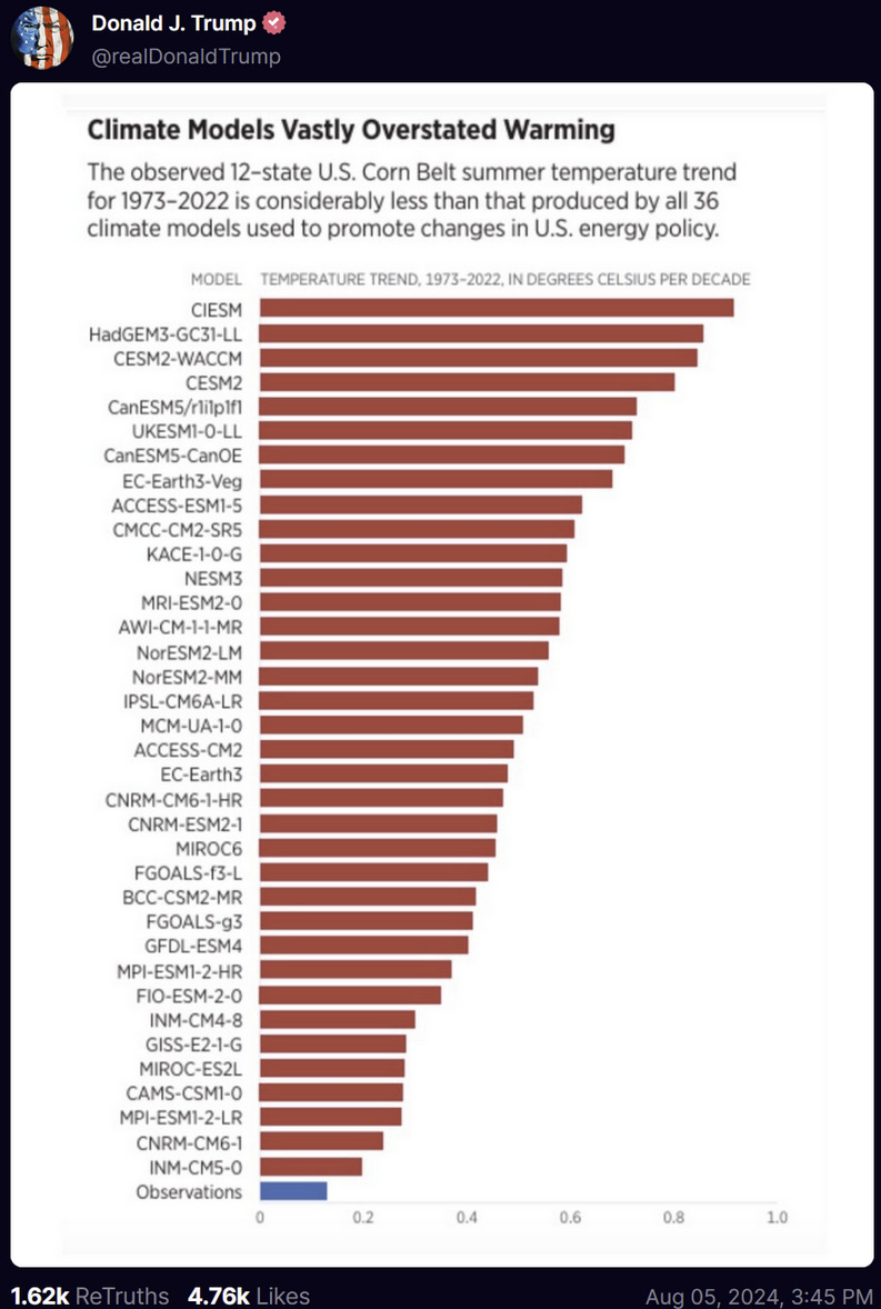
Today, it’s the claim that the models are hot and future warming will be much less than they predict. The source is some internet weirdo named Derwood Turnip, who posted this:
First, let’s be clear: climate models have an admirable track record of predicting the global average temperature. Zeke wrote a paper about that and it’s worth bookmarking so you’re ready to respond to anyone who says models are bad.
But Derwood’s post is about regional and seasonal climate change. While there are few details provided in the source document, I was able to reproduce the general result presented. So does this mean that models are warming too much?
What’s the problem with regional comparisons?
While the global average temperature is well constrained by planetary energy balance, how that warming is distributed around the planet can vary greatly due to what we refer to as unforced variability. This phenomenon is similar to the randomness we observe in weather patterns, but are driven by the ocean circulation on much longer time scales, such as the El Niño/La Niña oscillations.
Unforced variability can warm one region while simultaneously cooling another, with such variations spanning decades. This long-term variability adds a layer of complexity to prediction of regional climate change, even as the global average warming trend is well constrained.
As an example, you can take a climate model and run it many times, with identical emissions of carbon dioxide, but with each run starting with a slightly different state of the climate system. For these runs, the global average temperature change is similar, but how the warming is distributed varies greatly:

In some of the ensemble members (e.g., C16, C28), the Southeast U.S. cools between 2010 and 2060, while in most others it warms. In some members (e.g., C4, C29, C40), the Pacific Northwest cools, while in most others it warms.
This has important implications for Derwood’s plot. To see this, let’s take a single model, in this case, ACCESS-ESM1-5, which has an ensemble of 40 historical runs in the CMIP6 archive. Each run has different initial conditions, so each run of the model will have a different pattern of warming and cooling, just like we see in the plot above.
Summertime central U.S. warming in this one model ensemble looks like this:
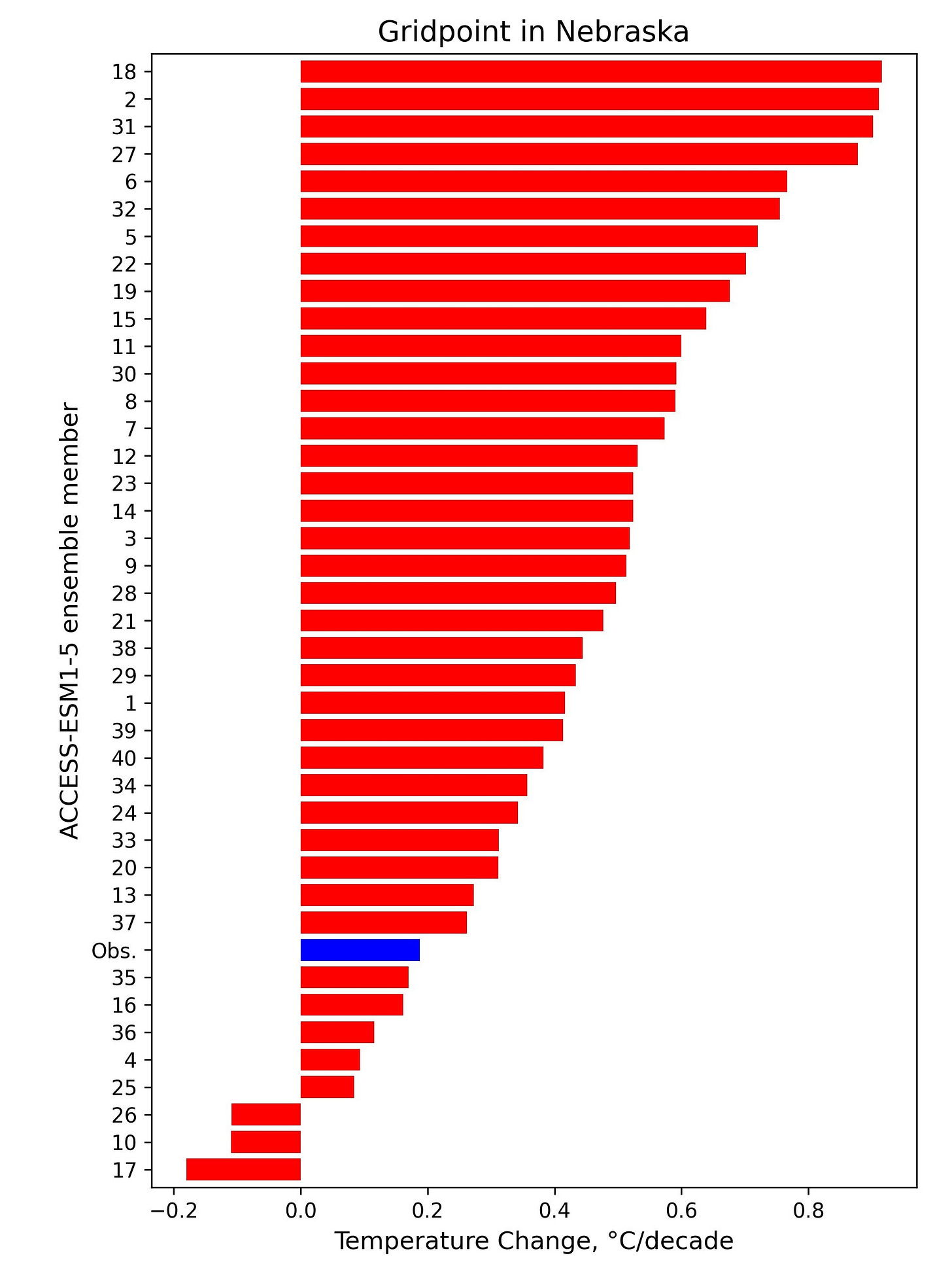
Wow! Unforced variability has a huge impact on what this model predicts. 20% of the runs show smaller warming than observations, and 8% show cooling. At the other end, there are ensemble members that show five times the observed warming. This spread is due entirely to different initial conditions, so this is an example of chaos in a strongly non-linear system.
So is the model overestimating warming or not? There’s no way to know. If you pick ensemble member 17, the model is underestimating the warming. If you pick ensemble member 35, the model is doing a fantastic job, while ensemble member 18 is overestimating the warming.
Without figuring out which of these ensemble members has unforced variability matching the unforced variability in the real world (this is really hard, by the way), the only correct conclusion is that the observed warming falls within the envelope of warming predicted by this model, so you cannot conclude that the ACCESS-ESM1-5 is overestimating warming.
This doesn’t mean that this model is right, of course. But it does mean that Derwood’s plot, which shows one value for this model, ~0.6°C, is bullshit. Probably not a surprise to anyone smart enough to read The Climate Brink.
To construct Derwood’s plot, I’m guessing a random run of each model was selected. So let’s remake Derwood’s plot, but using the ensemble member from each model that shows the lowest warming in this region. I limit myself to models that have ensembles with at least five runs in the CMIP6 archive.
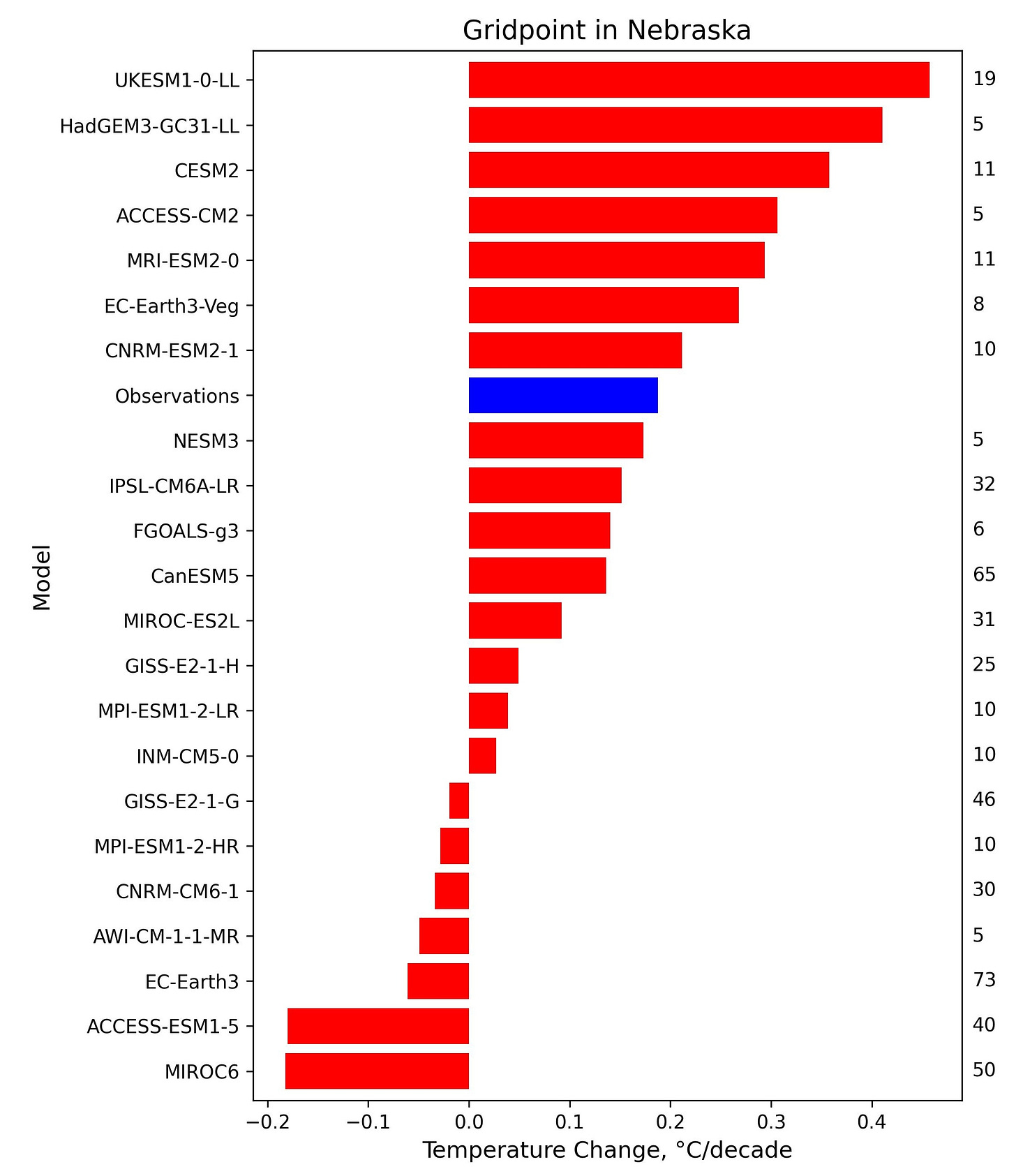
This shows that the results of the ACCESS-ESM1-5 are generalizable. Two thirds of the CMIP6 models produce warming lower than observations in their ensembles. Again, this doesn’t prove the models are right, but it does say that naive comparisons that ignore unforced variability, like Derwood’s plot, should not be taken seriously.
What’s a better way to do the calculation?
While unforced variability can impact any single location, if you look globally, the impact of it cancels out — regions that are cooled by unforced variability are cancelled by other regions that are warmed. Thus, the right way to do this calculation is globally.
To that end, I’ve taken a single (random) run of each of the 45 CMIP6 models and the observations and calculated this same change in summertime surface temperature, but at each point on the globe.
If the CMIP6 models are accurately simulating the climate, I would expect that areas where the model average is warming faster than the observations would be about equal to the area where the model average is warming slower.
In reality, the average warming in the CMIP6 models exceeds observed warming over 63% of the area of the Earth. This is larger than our expected 50%, but it is consistent with analyses showing that a subset of CMIP6 models does appear to be running too hot.
If we eliminate these too-hot models by screening out the models that have equilibrium climate sensitivity that’s out of the accepted range (2C-4C)1, then the average warming of the models exceeds observations over 48% of the area of the Earth, with observed warming exceeding the models over the other 52%.
This is exactly what we would expect if the models are accurately simulating the climate system.
What’s really going on?
This plot below shows the difference between the average of the screened model ensemble and the observations. Red colors indicate where the average model warming is faster than observations while blue areas show that models are warming slower. As mentioned above, 52% of the globe is blue, indicating places where the models are warming slower than observations.
The box over North America shows the region that Derwood’s plot focuses on.
[very John Mulaney voice] It’s weird … isn’t it weird … it’s weeeirrrd … that the region they picked just happens to be the place in the Northern Hemisphere where models look the absolute worst?
I have two comments on the selection of this region. First, I think it’s useful to understand the provenance of this plot. It comes from Dr. Roy Spencer via the Heritage Foundation. I won’t discuss in detail my tortured history with Roy other than to say that, when I see a scientific result from him, my baseline assumption is that he’s dishonestly manipulated the analysis to downplay the seriousness of climate change2.
In this case, it looks to me like Spencer intentionally selected this particular region to make models look bad. If so, it wouldn’t be the first time he’s done something like that. In a 2011 paper, I criticized Spencer for doing something similar:
There are three notable points to be made. First, [Spencer and Braswell] analyzed 14 models, but they plotted only six models and the particular observational data set that provided maximum support for their hypothesis. Plotting all of the models and all of the data provide a much different conclusion.
I can't read Spencer's mind to say for certain that he did this knowingly. However, the fact that he pinpointed the exact location where models perform the worst seems like too much of a coincidence to be anything other than intentional. But I’ll leave it to each of you to make that judgment for yourself.
The other comment is that, in addition to unforced variability, this is a region where other odd things are going on. Here are two papers that talk about why this region is warming less than expected during summertime. It turns out that this is the most agriculturally productive region on the planet, and land-use changes over the last few decades have largely offset greenhouse gas warming here.
To the extent that models have problems in this very small region, it’s much more likely to be connected to how well the models are handling land-use changes, not how well they represent global warming.
Models are actually good
Over my career, I've devoted considerable effort to comparing climate models with observations and have concluded that climate models perform surprisingly well, even on things I wouldn’t expect them to.
The saying “all models are wrong, but some are useful” applies here — climate models are far from perfect, but they are also incredibly informative. Most of the criticisms of models are based on bogus, misleading analyses. This one is no exception.
Update: a loyal reader pointed out that Gavin Schmidt made many of these same points on RealClimate in January. It’s an excellent write-up so go read it.


Derwood may be put into a position to make climate policy. If not computer models, what predictive tool was he planning to use to evaluate that policy before implementing it? Crystal Ball? Ouija Board? Tea leaves? Chicken bones? Asking for a friend.
ubrew12 @1,
Your friend should rest assured that his crystal ball, ouija board and morning cuppa are all safe. Even Foghorn Leghorn can sleep easy in his bed. The fake human 'Derwood Turnip' obtains the best divinations ever in history and he uses other means.
In the case of the corn state summer tmperatures, there is a bit of a disconnect between 'Derwood Turnip' and the information he presents. The actual author is the blunderful denialist Roy Spencer who posted an analysis on his blog in June 2023 and then included it in a pack of nonsense he had published in January 2024 by a bunch called The Heritage Foundation. It took 'Derwood Turnip' eight months to re-post the published graphic.
Such delay is something 'Derwood Turnip' has a history of creating. An example of a shorter 82-hour delay 'Derwood Turnip' created back in 2019 involved Hurricane Dorian, initially a Cat-5 hurricane but soon to be dropping to Cat-2. 'Derwood Turnip' used his position as POTUS and his very own exceptional analytical skills to give warning to the good citizens of Alabama (and others) that they "will most likely be hit (much) harder than anticipated" by Hurricane Dorian which was "looking like one of the largest hurricanes ever."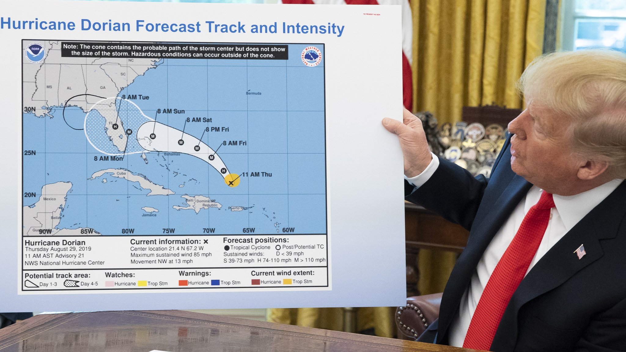
Yet during this 82-hour delay, the situation with Hurricane Dorian had changed dramatically. Advisory #021 had been updated multiple times (as is normal, with updates 4-times-a-day), having been superceded by Advisory #032A three hours prior to the warning of 'Derwood Turnip'.
The enormity of the wisdom of 'Derwood Turnip' can be seen in his detailed explanation for the remarkable variance between his wondrous analysis and the reality he so often wrestles with.
This article includes a graph of the worlds 1970-2023 prediction anomaly. This is pure speculation, but the anomaly in question may not be simply 'unforced variability'. We know that in the 30 years before 1970, the Corn Belt was recovering from the 'Dust Bowl': non-evaporative fallow land was being replaced by irrigated crops. Post 1970 this trend would have continued, as better agricultural practices filled the summer Corn Belt with evapotranspirating crops: a form of human agency the climate models may not include as a boundary condition. If so, then such a overprediction anomaly may also be found in other cropland areas, like in Ukraine.
An opposite effect might be expected in places where evapotranspirating jungle was, post 1970, being cut down and replaced with relatively inefficient ranchlands, soybeans, and palm oil plantations: Brazil and Borneo. Hence, they show up colored blue in that graph.
I'm just speculating. Do the climate models account for this kind of human agency, land-use change, as a boundary condition?
ubrew12 @3,
The models do certainly calculate soil moisture and account for surface albedo. I don't know how accurately this is done. Presumably, if it were done badly enough to affect the modelling generally, such a failing would be quickly corrected.
You ask this because you wonder whether the 'Dust Bowl' could be the reason for these Corn Belt states having seen such low warming rates 1973-2022. Perhaps they began the period with warming already in place.
The GISTEMP web site easily allows such ideas to be tested. Over the full 1880-2022 period of data, the same low warming trend is still seen across the eastern USA thro' summer months on a global map. It is actually there all year and strongest in Autumn,weakest in Winter & Spring. So using this region to be representative of AGW, it is simply a dishonest cherry-pick (which is what 'Derwood Turnip' is doing). And as a region testing the climate models, as shown in the global map above in the OP, it is again a dishonest cherry-pick (which is what Roy Spencer is doing), although Montana/North Dakota would give a more dramatic result, indeed the most dramatic result.
ubrew12:
As MA Rodger says, climate models do include soil moisture and surface albedo. The surface component of these models will also include vegetation cover, as this strongly influences the evapotranspiration rates. This is an essential part of the climate modelling process, as the surface energy balance has major implications in partitioning energy within the climate system.
The surface energy balance involves:
The concept of a "surface energy balance" is based on the idea that the surface is an infinitely thin plane that separates the atmosphere and the earth (land/sea). With no thickness, it has no mass, so it cannot store energy. There must be an energy balance that sums to zero for all energy flows to or from the surface. In this concept, the land itself is the sub-surface (which can store energy).
NCAR has a good web page describing their models. The overall climate model is built from several components: atmosphere, land, ice, etc. For the land component, the docuimentation table of contents lists (under "special cases") things like "Running the prognostic crop model" and "Running with irrigation".
So yes, it is possible to run these models with various aspects of surface conditions. Whether anyone has is another question - and getting appropriate historical surface data to do so accurately is an even bigger question.