Posted on 31 January 2014 by dana1981, Rob Painting, John Cook

A number of studies, both regional and global, have found that heatwaves are becoming more frequent. According to research by climate scientists David Karoly and Sophie Lewis, Australian heatwaves in the last decade are at least five times more likely than in the 20th century. Similarly, in the USA, Meehl (2009) examined how the ratio of hot to cold records in the United States and found that more and more local heat records are being broken (Figure 5).

Figure 5: Ratio of record daily highs to record daily lows observed at about 1,800 weather stations in the 48 contiguous United States from January 1950 through September 2009. Each bar shows the proportion of record highs (red) to record lows (blue) for each decade. The 1960s and 1970s saw slightly more record daily lows than highs, but in the last 30 years record highs have increasingly predominated, with the ratio now about two-to-one for the 48 states as a whole.

Big changes at the extremes

As detailed in the SkS post on the freak 2010 Moscow heatwave, global temperatures follow what is called a Gaussian or normal distribution. That is, if you plot temperature series along two axes their frequency or density (vertical axis) and how far these temperature measurements deviate from the average (horizontal axis), will tend to be clustered around the average. These observations or values resemble a bell-shaped curve. See figure 2.  

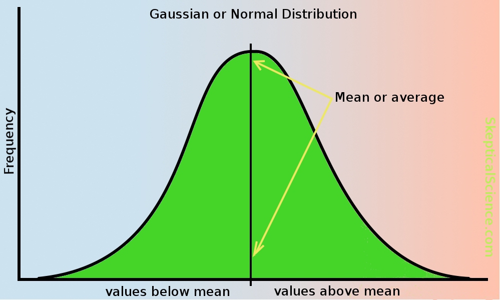
Figure 2 - illustration of a Normal/Gaussian distribution

Not all climate-related phenomena follow this Gaussian distribution, but a number of studies show that surface temperatures do. Intuitively this makes sense, because although surface temperatures can exhibit large swings from time to time they generally don't deviate much from the average throughout the year.

Because of the shape of this distribution, one can mathematically determine the spread of the values. This is known as the 68-95-99.7, three-sigma, or empirical rule, where the percentage of a particluar value declines as one moves further away from the mean. 68.2% of all values are within one standard deviation of the mean, 95.4% within two standard deviations, and 99.7% within 3 standard deviations. See figure 3, and note the greek symbol is sigma representing a standard deviation.

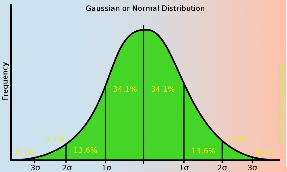
Figure 3 - Gaussian distribution with standard deviations.

With a warming climate the mean temperature begins to slowly climb too, so the bell-shaped curve creeps to the right in the warming direction (figure 4). As it does so, you can see how it affects the measurements at the extremes - warm extreme temperatures become more common place, and cold extremes less common. A shifting mean (as in warming global temperatures) leads to large changes at the extremes.  

Fig 4 - illustration of gaussian distribution with a shifting mean.

Rahmstorf & Coumou 2011

Rahmstorf and Coumou (2011) developed a statistical model and found that record-breaking extremes depend on the ratio of trend (warming or cooling) to the year-to-year variability in the record of observations. They tested this model by analysing global temperatures and found that warming increased the odds of record-breaking. When applied to the July 2010 temperatures in Moscow, they estimated a 80% probability that the heatrecord would not have occurred without climate warming.

Figure 1 - Probability of July average temperature anomalies in Moscow, Russia since 1950. This image shows that the average temperature in Moscow for July 2010 was significantly hotter than in any year since 1950. Credit: Claudia Tebaldi and Remik Ziemlinski. From ClimateCentral.org

Some statistical background

Earlier statistical work on record-breaking events has shown that for any time series that is stationary (i.e. no trend), the probability of record-breaking falls with each subsequent observation. This is known as the 1/n rule, where n equals the previous number of data in the series. For example, the first observation has a 1-in-1 chance of being the record extreme (100%), the second has a 1-in-2 chance (50%), the third a 1-in-3 chance, and so on.

For climate heat records, the stationarity rule is not apparent, as one might expect in a warming world. Previous work in this area has shown that the slowly warming mean (average) temperature is responsible for this nonstationarity.   

Monte Carlo 

Following on from this earlier work, Rahmstorf and Coumou (2011) sought to disentagle the two effects of the mean change in temperature (climate warming), from the random fluctuations of weather, so as to find out the contribution of each to record-breaking. To do this, the study authors turned to Monte Carlo simulations. These are computer-generated calculations which use random numbers to obtain robust statistics. A useful analogy here is rolling a dice. Rolling once tells us nothing about the probability of a six turning up, but roll the dice 100,000 (as in this experiment) and you can calculate the odds of rolling a six. 

From the simulations the authors obtain 100 values which represent a 100 year period. Figure 2(A) - 2(C) are the "synthetic" time series, and 2(D), 2(E) are respectively, the 'synthetic' global mean and Moscow July temperature. In all panels the data have been put into a common reference frame (nomalized) for comparison. (See figure 1 for an example of a Gaussian or normal distribution. Noise represents the year-to-year variability). 

Figure 2 - examples of 100 year time series of temperature, with unprecedented hot and cold extremes marked in red and blue. A) uncorrelated Gaussian noise of unit standard deviation. B) Gaussian noise with added linear trend of 0.078 per year. C) Gaussian noise with non-linear trend added (smooth of GISS global temp data) D) GISS annual global temp for 1911-2010 with its non-linear trend E) July temp at Moscow for 1911-2010 with non-lneartrend. Temperatures are normailzed with the standard deviation of their short-term variability (i.e. put into a common frame of reference). Note: For the Moscow July temperature (2E) the long-term warming appears to be small, but this is only because the series has been normalized with the standard deviation of that records short-term variability. In other words it simply appears that way because of the statistical scaling approach - the large year-to-year variability in Moscow July temperatures makes the large long-term increase (1.8°C) look small when both are scaled. Adapted from Rahmstorf & Coumou (2011)

Follow steps one.....

Initially, the authors ran the Monte Carlo simulations under 3 different scenarios, the first is for no trend (2[A]), with a linear trend (2[B]) and a nonlinear trend (2[C]). The record-breaking trends agree with previous statistical studies of record-breaking namely that: with no trend the probability of record-breaking falls with each observation (the 1/n rule), and with a linear trend the probability of record-breaking gradually reduces until it too exhibits a linear trend. With a non-linear trend (2[C]), the simulations show behaviour characteristic of the no-trend and linear trend distibutions. Figures 2(D) and 2(E) are the actual GISS global and Moscow July temperatures respectively.

.....two.....

Next, the authors then looked at both the GISS global and Moscow July temperature series to see whether they exhibited a gaussian-like distribution (as in the 'lump' in figure 1). They did, so this supports earlier studies  indicating that temperature deviations are fluctuating about, and shifting with a slowly moving mean (as in the warming climate). See figure 3 below.   

Figure 3 -Histogram of the deviations of temperatures of the past 100 years from the nonlinear climate trend lines shown in Fig. 2(D)  and (E) together with the Gaussian distributions with the same variance and integral. a) Global annual mean temperatures fromNASA GISS, with a standard deviation of 0.088 ºC. (b) July mean temperature at Moscow station, with a standard deviation of 1.71 ºC. From Rahmstorf & Coumou (2011)

.....and three.

Although the authors calculate probabilities for a linear trend, the actual trend for both the global, and Moscow July temperature series is nonlinear. Therefore they separated out the long-term climate signal, and the weather-related annual temperature fluctuation, which gave them a climate 'template' on which to run Monte Carlo simulations with 'noise' of the same standard deviation (spread of annual variability from the average, or mean). This is a bit like giving the Earth the chance to roll the 'weather dice' over and over again.

From the simulations with, and without the long-term trend, the authors could then observe how many times a record-breaking extreme occurred.

Figure 4 -Expected number of unprecedented july heat extremes in Moscow for the past 10 decades. Red is the expectation based on Monte Carlo simulations using the observedclimate trend shown in Figure 2(E). Blue is the number expected in a stationary climate (1/n law). Warming in the 1920's and 1930's and again in the last two decades increases the expectation of extremes during those decades. From Rahmstorf and Coumou (2011)

Large year-to-year variability reduces probability of new records

A key finding of the paper was that if there are large year-to-year non-uniform fluctuations in a set of observations with a long-term trend, rather than increasing the odds of a record-breaking event, they act to reduce it because the new record is calculated by dividing thetrend by the standard deviation  The larger the standard deviation the smaller the probability of a new extreme record.

This can be seen by comparing the standard deviation of the NASA GISS, and Moscow July temperature records (figure 3), plus figure 2(D) and [E]). As the GISS global temperature record has a smaller standard deviation (0.088°C) due to the smaller year-to-year fluctuations in temperature, you will note in figure 2(D) that it has a greater number of record-breaking extremes than the Moscow July temperature record over the same period (2[E]). So, although the long-term temperature trend for Moscow in July is larger (100 yeartrend=1.8°C), so too is the annual fluctuation in temperature (standard deviation=1.7°C), which results in lower probability of record-breaking warm events. 

Interestingly it's now plain to see why the  MSU satellite temperature record, which has a large annual variability (large standard deviation, possibly from being overly sensitive to La Niña & El Niño atmospheric water vapor fluctuations) still has 1998 as it warmest year, whereas GISS has 2005 as it's warmest year (2010 was tied with 2005, so is not a newrecord). Even though the trends are similar in both records, the standard deviation is larger in the satellite data and therefore the probability of record-breaking is smaller. 

Coumou Guardian post

Dim Coumou and Alexander Robinson from the Potsdam Institute for Climate Impact Research have published a paper in Environmental Research Letters (open access, free to download) examining the frequency of extreme heat events in a warming world.

They compared a future in which humans continue to rely heavily on fossil fuels (an IPCC scenario called RCP8.5) to one in which we transition away from fossil fuels and rapidly reduce greenhouse gas emissions (called RCP2.6). In both cases, the global land area experiencing extreme summer heat will quadruple by 2040 due to the global warming that's already locked in from the greenhouse gases we've emitted thus far.

However, in the low emissions scenario, extreme heat frequency stabilizes after 2040 (left frames in Figure 1), while it becomes the new norm for most of the world in the high emissions, fossil fuel-heavy scenario (right frames in Figure 1) (click here for a larger version).

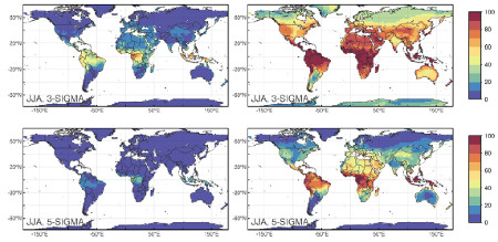Figure 1: Multi-model mean of the percentage of boreal summer months in the time period 2071–2099 with temperatures beyond 3-sigma (top) and 5-sigma (bottom) under low emissions scenario RCP2.6 (left) and high emissions RCP8.5 (right).

Coumou & Robinson looked at the frequency of rare and extreme (3-sigma, meaning 3 standard deviations hotter than the average) and very rare and extreme (5-sigma) temperature events. 3-sigma represents a 1-in-370 event, and 5-sigma is a 1-in-1.7 million event.

As shown in the video below from NASA, summer temperatures have already begun to shift significantly towards more frequent hot extremes over the past 50 years. What used to be a rare 3-sigma event has already become more commonplace.

Summer temperatures shifting to hotter averages and extremes between the 1950s and 2000s. Source: NASA/Goddard Space Flight Center GISS and Scientific Visualization Studio

Coumou & Robinson point out that these 3-sigma events have tended to have very damaging consequences:

"most of the 3-sigma extremes that have occurred in recent years resulted in serious impacts to society, causing many heat-related deaths, massive forest fires or harvest losses"

Coumou pointed to the Moscow summer heat wave of 2010 as a good example of a damaging 3-sigma extreme heat event. Thousands died during that heat wave, and the associated drought cut Russia's wheat crop by 40 percent, cost the nation $15 billion, and led to a ban on grain exports, causing food prices to rise globally.

"In the Moscow region the average temperature for the whole of July was around 7°C [13°F] warmer than normal – it was around 25°C [77°F]. In some parts, temperatures above 40°C [104°F] were measured"

As Figure 1 above shows, if we continue to rely heavily on fossil fuels (right frames), these extreme heat events will occur throughout the summer for most of the global land area by the late 21st century, especially in the tropics. Currently, around 5 percent of the world's land mass is experiencing a 3-sigma event at any one time during the summer months.

In the high greenhouse gas emissions scenario, most of Africa, Central America, and northern South America will experience 3-sigma extreme heat events for close to 100 percent of the summer. They will become the norm. Even extreme 5-sigma heat events, which are currently exceptionally rare, will become relatively commonplace, especially near the equator.

On the other hand, in the scenario where we take major steps to reduce human greenhouse gas emissions (left frames in Figure 1), 3-sigma events will still be relatively rare by the late 21st century, especially outside of the tropics. Extreme 5-sigma events will become somewhat more commonplace near the equator, but will remain fairly rare occurrences globally.

In short, damaging summer extreme heat events are going to become more commonplace, but just how much more commonplace is up to us. While it's difficult to determine how climate change will impact some types of extreme weather (tornadoes, for example), the link between global warming and heat waves is quite clear. Increasing global temperatures will make (and have already made) extreme heat events more commonplace.

The longer we continue to rely on fossil fuels and the higher our greenhouse gas emissions, the more extreme heat we'll lock in. If we manage to take serious action to reduce our greenhouse gas emissions, we can limit global warming to a level where extreme heat events will become more commonplace, but to a level we can manage to adapt to.

If we continue our reliance on fossil fuels and associated greenhouse gas emissions growth, we'll commit ourselves to a world where today's most extreme heat waves become the norm, and future extreme heat makes today's heat waves look downright balmy.

It's in our hands which future scenario becomes reality. It's like one of those choose your own adventure books, but real. Which future will we choose?

Coumou on increasing heatwaves

A new paper published in Climatic Change by Coumou, Robinson, and Rahmstorf (CRR13) finds that record-breaking monthly temperature records are already occurring five times more often than they would in the absence of human-caused global warming. There is an 80% chance that any monthly heat record today is due to human-caused global warming.

They examined the increased frequency of record-breaking monthly temperature records over the past 130 years, finding that these records are now five times more likely to occur due to global warming, with much more to come.

"...worldwide, the number of local record-breaking monthly temperature extremes is now on average five times larger than expected in a climate with no long-term warming. This implies that on average there is an 80% chance that a new monthly heat record is due to climatic change ... Under a medium global warming scenario, by the 2040s we predict the number of monthly heatrecords globally to be more than 12 times as high as in a climate with no long-term warming."

Figure 1: Observed record ratio (the increase in the number of heat records compared to those expected in a world without global warming) for monthly heat records as it changes over time (thin red line is annual data, thick red line smoothed with half-width 5 years). This is compared with predictions from a simple stochastic model based only on the global mean temperature evolution (blue line with uncertainty band directly comparable to the smoothed red curve)

CRR13 considers the formula for the probability of a record-breaking extreme in a Gaussian(bell curve) time series with a linear long-term warming trend, compared to the much more simplified version of the same formula when there is no warming trend.  The paper then examines the ratio of those two equations - the increased frequency of record-breaking extreme heat events in a warming world.

The study uses global surface temperature data provided by the NASA Goddard Institute for Space Studies (GISS) for 1880–2010, in 2° by 2° grids across the globe, excluding polarregions above 70° latitude due to the sparse temperature station coverage there  They examine the temperature data for each calendar month of the year.

CRR13 finds that the number of observed heat records is much larger than one would have expected in a climate with no long term warming, and many monthly heat records have been broken over the past decade.

In Figure 2 below, the increase in observed monthly heat records in the past decade over the most recent 40-year period of data (left column) are compared to the modeled results (right column) for northern hemisphere summer (top row), winter (middle row), and the whole year (bottom row).

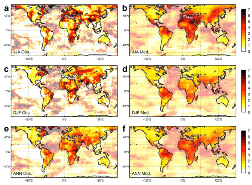
Figure 2: Global maps of the observed record ratio (the increase in the number of heatrecords compared to those expected in a world without global warming) as observed (left panels) and estimated by the model (right panels) using the 1971–2010 dataset. a and bshow boreal summer results (June-July-August), c and d austral summer results (December-January-February) and e and f results for all months.

Figure 3 looks at the increase in heat records over the past decade as compared to the full 131-year dataset. The similarity between Figures 2 and 3 shows that over the past decade, the monthly records in the past decade as compared to the past 40 years are usually also records as compared to the past 131 years.

The bottom right panel (d) also shows the probability that a monthly heat record in a given location is due to global warming, with blue indicating 0% probability and red indicating 100%.

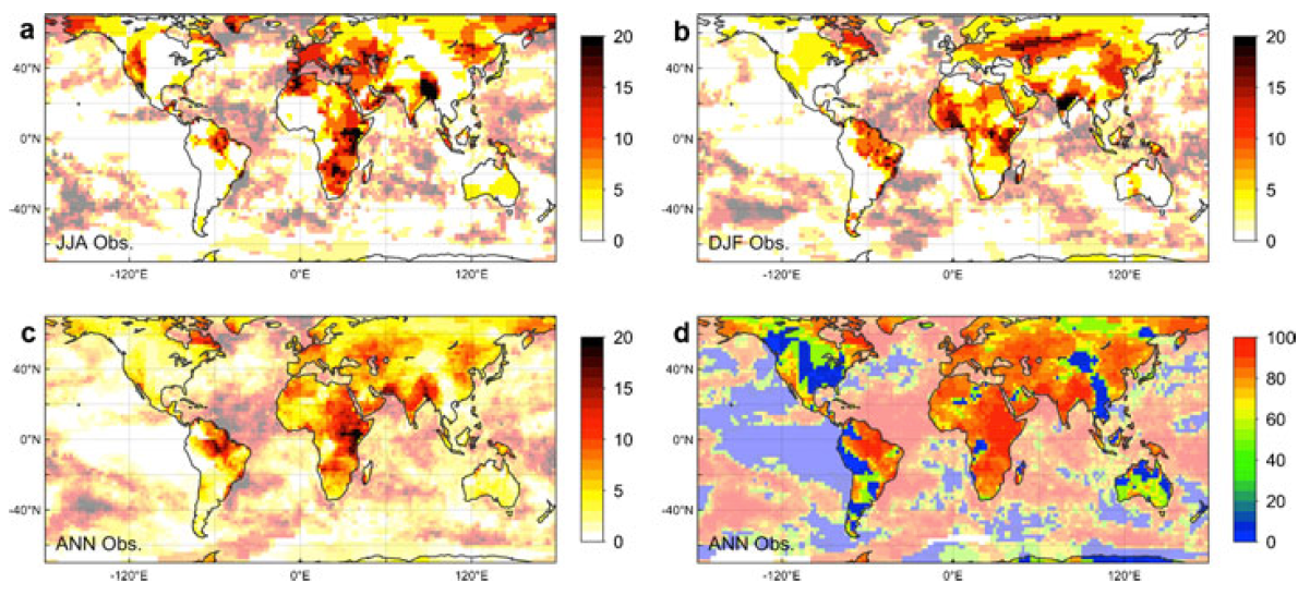
Figure 3: Global maps of the observed record ratio over the past decade (the increase in the number of heat records compared to those expected in a world without global warming) over the 1880–2010 dataset, for a boreal summers (June-July-August), b austral summers (December-January-February) and c all months. d Risk map showing the probability that a record-breaking event in the last decade is due to climatic change.

In Figure 1 above, CRR13 extends the model forward assuming global warming based on a moderate emissions scenario, Representative Concentrations Pathway (RCP) 4.5, in which human greenhouse gas emissions peak around the year 2040, ultimately causing aradiative forcing (global energy imbalance) of 4.5 Watts per square meter in 2100 (a doubling of atmospheric CO2 would cause a forcing of about 3.7 Watts per square meter).  This scenario would ultimately lead to about 3.6°C global surface warming above pre-industrial levels, which is a very dangerous and possibly catastrophic amount of global warming, but certainly not a worst case scenario.  It essentially represents a scenario where we take too-slow and gradual action to reduce human greenhouse gas emissions, and at the moment seems fairly realistic.

In this scenario, CRR13 finds that by 2040, monthly heat records will have become approximately 12 times more likely to occur than in a non-warming world,

"...approximately 80% of the recent monthly heat records would not have occurred without human influence on climate. Under a medium future global warming scenario this share will increase to more than 90% by 2040."

As lead author Coumou noted, this is even worse than it sounds, because breaking a heatrecord in 2040 will require much higher temperatures than breaking a record today.

"Now this doesn’t mean there will be 12 times more hot summers in Europe than today – it actually is worse.  To count as new records, they actually have to beat heat records set in the 2020s and 2030s, which will already be hotter than anything we have experienced to date.  And this is just the global average – in some continental regions, the increase in new records will be even greater."

Donat and Alexander find 40% increase in extreme temperatures

Donat and Alexander 2012 (DA12) examined changing temperature distributions globally. DA12 used HadGHCND, a global gridded data set of observed near-surface daily minimum and maximum temperatures from weather stations, available from 1951 and updated to 2010.  Using this dataset, DA12 calculated probability distribution functions using daily temperature anomalies for 1951–1980 and 1981–2010.  They then calculated the frequency of temperature anomaly ranges by using bin widths of 0.5°C and binning counts of temperature anomalies between -25 and +25°C.

DA12 first investigated how the temperature distribution mean, variance, and skewness (asymmetry) have changed between the two 30-year periods geographically, for both minimum and maximum temperatures (Figure 1).

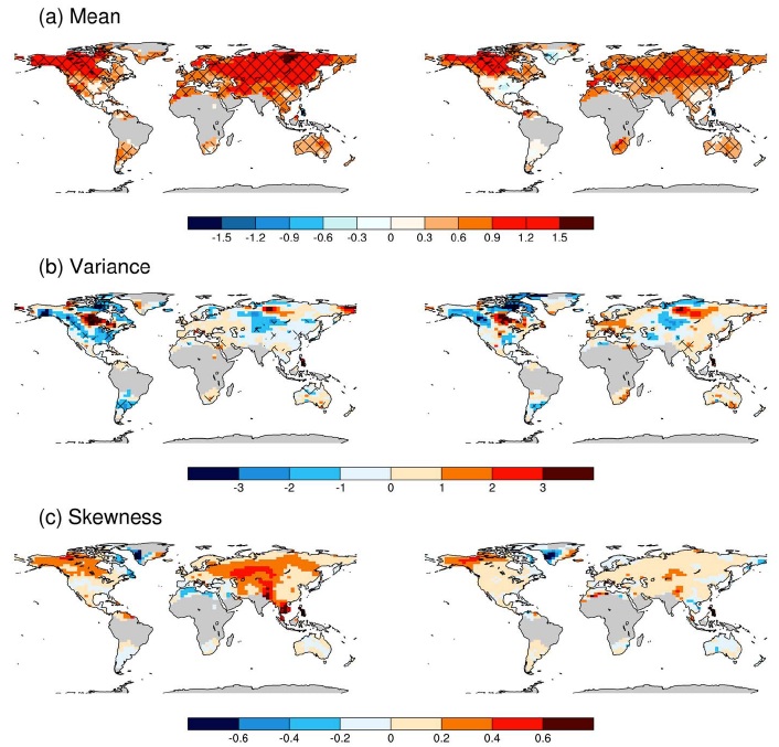
Figure 1: The differences in higher moment statistics of (a) mean, (b) variance, and (c) skewness for each grid box in HadGHCND for (left) daily minimum temperature anomalies and (right) daily maximum temperature anomalies for the two time periods shown. Hatching indicates changes between the two periods that are significant at the 10% level for the mean (using a Student’s t-test) and the variance (using an f-test) of the distribution.  From Donat and Alexander 2012.

DA12 found that the distributions of both minimum and maximum temperatures have shifted towards warming temperatures almost everywhere on the planet. They also found that in most regions, the skewness of the distribution has shifted towards hotter temperatures (Figure 2).  However, the change in variance in the data is less geographically consistent. 

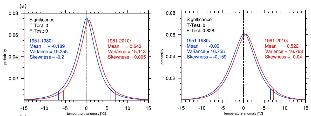
Figure 2: Probability density functions for two periods 1951–1980 (blue) and 1981–2010 (red) of anomalies of (left) daily minimum temperature and (right) daily maximum temperature. Statistics related to the shape, scale and location parameters are also shown. The distribution functions are presented for the globe.  The vertical lines represent the 5th and 95th percentiles of the respective distribution.  Figure 2a from Donat and Alexander 2012.

The authors found that the shifting temperature distribution has made extreme heat waves much more likely to occur now than in the middle of the 20th Century (emphasis added):

"This increases extreme temperatures in such a way that the 95th percentile of the first period is the 92.7th percentile of the second period (i.e., there is a 40% increase in more recent decades in the number of extreme temperatures defined by the warmest 5% of the 1951–1980 distribution)."

Hansen et al find shift towards heatwaves

Hansen et al. examined the surface temperature record to determine how the distribution of temperatures has changed over the past six decades.  As we know, the average global temperature has increased approximately 0.7°C over that period, so not surprisingly, the distribution of temperature anomalies has also shifted towards warmer values on average, as illustrated by the animation below and Figure 1.

Source: NASA/Goddard Space Flight Center GISS and Scientific Visualization Studio 

This main conclusion that we are seeing more and stronger heat waves as a consequence of global warming is a clear, expected, empirical result which we would hope nobody will dispute.  The controversy comes in when these results are used to try and attribute individual heat waves to human-caused global warming.

Otto on Russian Heatwave

Otto et al. (2012) examined whether the 2010 extreme Russian heat wave could be attributed to human influences. The 2010 Russian heat wave was also previously investigated by Dole et al. (2011) andRahmstorf and Coumou (2011).  The conclusions of the two papers seemed contradictory - Dole et al. found:

"that the intense 2010 Russian heat wave was mainly due to natural internal atmospheric variability"

Whereas like Hansen et al., Rahmstorf and Coumou concluded that humans played a role in the Russian heat wave:

"For July temperature in Moscow, we estimate that the local warming trend has increased the number of records expected in the past decade fivefold, which implies an approximate 80% probability that the 2010 July heat record would not have occurred without climate warming."

However, Otto et al. note that these two conclusions are not necessarily contradictory, and can even be considered complementary.

First, Otto et al. examined the local temperature record in Western Russia and found from 1950 to 2009, it warmed 1.9 +/- 0.8 times the rate of global warming, with approximately 1°C local warming over that timeframe (Figure 3).

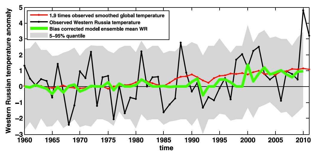
Figure 3: Modeled and observed temperature anomalies averaged over 50°–60°N, 35°–55°E. Also shown is the smoothed global mean temperature multiplied by the regression coefficient of Western Russian temperatures. The reference period is 1950–2009 for observed data and 1960–2009 for the model.  Figure 1 in Otto et al. (2012).

Otto et al. then used use the global circulation model HadAM3P to simulate Russian temperature changes in order to determine how frequently extreme heat waves can be expected to occur during current hotter temperatures as opposed to the cooler 20th Century (Figure 4).

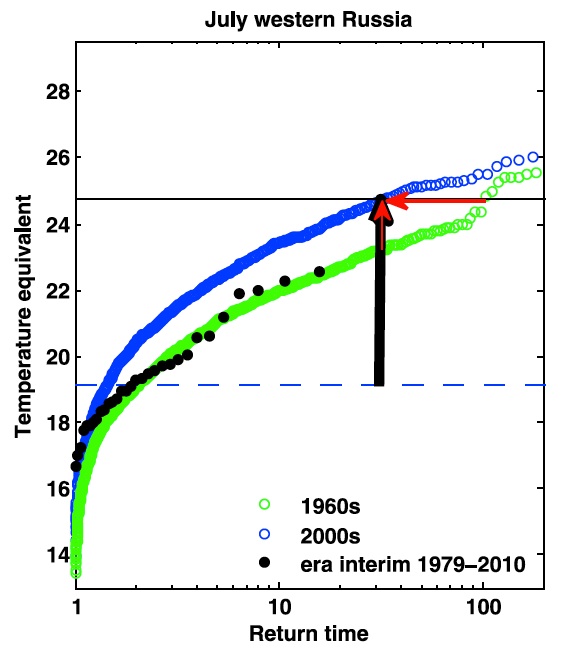
Figure 4: Return periods of temperature-geopotential height conditions in the model for the 1960s (green) and the 2000s (blue) and in ERA-Interim for 1979-2010 (black). The vertical black arrow shows the anomaly of the Russian heat wave 2010 (black horizontal line) compared to the July mean temperatures of the 1960s (dashed line). The vertical red arrow gives the increase in the magnitude of the heat wave due to the shift of the distribution whereas the horizontal red arrow shows the change in the return period.  Figure 4 in Otto et al. (2012).

The "return time" on the Figure 4 x-axis tells us how frequently the model simulates that the temperatures on the y-axis will occur for 1960s Russian temperatures (green) and 2000s Russian temperatures (blue).  So for example, in the 2000s a temperature equivalent of 24.5 occurs once every 33 years in the model.

The vertical black arrow shows the difference between the horizontal dashed blue line (average 1960s Russian temperature) and the horizontal black line (the 2010 Russian heatwave).  The vertical red arrow shows the difference between modeled Russian temperature distributions in 1960 and 2010, the difference being primarily due to human-caused warming.  And the horizontal red arrow shows the difference between the frequency that the 2010 Russian heat wave occurred during modeled 1960 and 2010 temperatures.  Otto et al. draw two key conclusions about 2010 Russian heat wave from these data:

• The heat wave was not entirely or even mostly human-caused, because the vertical black arrow is much larger than the vertical red arrow.  In this sense Dole et al. are right.

• The heat wave is now three times more likely to occur (now a 1-in-33 year event vs. a 1-in-99 year event in the 1960s).  In this sense Hansen et al. and Rahmstorf and Coumou are correct.

So ultimately Otto et al. find that the conclusions of these papers are not contradictory, but complementary.  While extreme heat events like the 2010 Russian event are by no means entirely human-caused, local and global warming have made them much more likely to occur.  As Hansen et al. noted, due to the shifting temperature distributions also discussed by DA12, heat waves are now hotter and more frequent than they were last century.

Zwiers et al. (2011):

"Therefore, it is concluded that the influence of anthropogenic forcing has had a detectable influence on extreme temperatures that have impacts on human society and natural systems at global and regional scales"

warning & myth

the significance of increasing risk from heatwaves is downplayed by the use of the For example, Hunt/Abbott argued:

QUOTE

This logical fallacy non sequitor (Latin for 'it does not follow'). This is a fallacy where the conclusion isn't supported by the premise. Its the equivalent of arguing that people have died of cancer long before cigarettes were invented, hence smoking can't cause cancer.

Conclusion

Unless we take steps to significantly reduce human greenhouse gas emissions and global warming, by 2040 the frequency of monthly heat records will become 12 times the rate in a non-warming world, and we will be able to blame more than 90% of heatrecords on global warming.

This would of course be bad news.  For example, as shown by Hawkins et al. (2012), crops tend not to respond well to extreme heat, so these findings could pose a significant problem for global food production, as well as increasing heat fatalities, requiring costly adaptive measures to prepare people for more frequent extreme heat waves.  In January of 2013,Australia has been trying to cope with this sort of extreme heat, which has resulted indevastating wildfires and other nasty consequences.