Climate Science Glossary

Term Lookup

Enter a term in the search box to find its definition.

Settings

Use the controls in the far right panel to increase or decrease the number of terms automatically displayed (or to completely turn that feature off).

Term Lookup

Settings


All IPCC definitions taken from Climate Change 2007: The Physical Science Basis. Working Group I Contribution to the Fourth Assessment Report of the Intergovernmental Panel on Climate Change, Annex I, Glossary, pp. 941-954. Cambridge University Press.

Home Arguments Software Resources Comments The Consensus Project Translations About Support

Twitter Facebook YouTube Mastodon MeWe

RSS Posts RSS Comments Email Subscribe


Climate's changed before
It's the sun
It's not bad
There is no consensus
It's cooling
Models are unreliable
Temp record is unreliable
Animals and plants can adapt
It hasn't warmed since 1998
Antarctica is gaining ice
View All Arguments...


Username
Password
New? Register here
Forgot your password?

Latest Posts

Archives

Monckton Myth #3: Linear Warming

Posted on 18 January 2011 by dana1981

In his recent response to Steketee's article in The Australian, Monckton's argument #5 reads as follows:

In the 40 years since 1970, global temperatures have risen at a linear rate equivalent to around 1.3 °C/century. CO2 concentration is rising in a straight line at just 2 ppmv/year at present and, even if it were to accelerate to an exponential rate of increase, the corresponding temperature increase would be expected to rise merely in a straight line. On any view, 1.3 °C of further “global warming” this century would be harmless. The IPCC is predicting 3.4 °C, but since the turn of the millennium on 1 January 2001 global temperature has risen (taking the average of the two satellite datasets) at a rate equivalent to just 0.6 °C/century, rather less than the warming rate of the entire 20th century. In these numbers, there is nothing whatever to worry about – except the tendency of some journalists to conceal them.

This paragraph contains a number of erroneous statements.  Firstly, according to both GISTEMP and HADCRUT3 (satellite data only began in 1979), the global temperature trend since 1970 is 1.6–1.7°C per century.  Secondly, the atmospheric CO2 concentration has been accelerating (not linear).  The rate of increase in atmospheric CO2 in the 2000's (2.2 parts per million by volume [ppmv] per year) was in fact 47% faster than the rate of increase in the 1990s (1.5 ppmv per year).  Monckton uses these incorrect assertions to create the support for his incorrect argument - that if we continue with business-as-usual, global temperatures over the next century will increase at a constant, linear rate (or slower).

Temperature Response to CO2

Monckton claims that an exponential increase in atmospheric CO2 concentration would result in a linear increase in global temperature.  But of course that depends on what the exponent is in the exponential increase.  Monckton is referring to the logarithmic relationship between radiative forcing (which is directly proportional to the change in surface temperature at equilibrium) and the atmospheric CO2 increase.  Note that we are not currently at equilibrium as there is a planetary energy imbalance, and thus further warming 'in the pipeline' from the carbon we've already emitted.  Therefore, estimates of the rate of warming due to CO2 thus far will will be underestimates, unless accounting for this 'warming in the pipeline' (which Monckton does not).

This logarithmic relationship means that each doubling of atmospheric CO2 will cause the same amount of warming at the Earth's surface.  Thus if it takes as long to increase atmospheric CO2 from 560 to 1120 ppmv as it did to rise from 280 to 560 ppmv, for example, then the associated warming at the Earth's surface will be roughly linear.  So the question then becomes, how fast do we expect atmospheric CO2 to rise over the next century?

How Fast will Atmospheric CO2 Rise?

The IPCC addressed this question by examining a number of different anthropogenic emissions scenarios.  Scenario A1F1 assumes high global economic growth and continued heavy reliance on fossil fuels for the remainder of the century.  Scenario B1 assumes a major move away from fossil fuels toward alternative and renewable energy as the century progresses.   Scenario A2 is a middling scenario, with less even economic growth and some adoption of alternative and renewable energy sources as the century unfolds.  The projected atmospheric CO2 levels for these scenarios is shown in Figure 1.

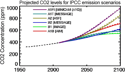
Figure 1: Atmospheric CO2 concentrations as observed at Mauna Loa from 1958 to 2008 (black dashed line) and projected under the 6 IPCC emission scenarios (solid coloured lines). (IPCC Data Distribution Centre)

In short, following the 'business as usual' approach which Monckton argues for, without major steps to move away from fossil fuels and limit greenhouse gas emissions, we will likely reach 850 to 950 ppmv of atmospheric CO2 by the year 2100.  It will have taken approximately 200 years (from 1850 to 2050) for the first doubling of atmospheric CO2 from 280 to 560 ppmv, but it will only take another 70 years or so to double the levels again to 1120 ppmv.  This will result in an accelerating rate of global warming, not a linear rate.  Under Scenarios A2 and A1F1, the IPCC report projects that the global temperature in 2095 will be 2.0–6.4°C above 1990 levels (2.6-7.0°C above pre-industrial), with a best estimate of 3.4 and 4.0°C warmer (4.0 and 4.6°C above pre-industrial average surface temperatures), respectively. 

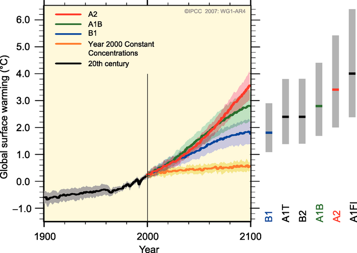
Figure 2: Global surface temperature projections for IPCC Scenarios. Shading denotes the ±1 standard deviation range of individual model annual averages. The orange line is  constant CO2 concentrations at year 2000 values. The grey bars at right indicate the best estimate (solid line within each bar) and the likely range.  (Source: IPCC).

Life in the Fast Lane

Monckton claims that these projected amounts of warming have not been borne out in the surface temperature changes over the past decade.  But there are many factors which impact short-term global temperatures, which may conceal the long-term warming caused by increasing atmospheric CO2.  So if we want to know if the IPCC projections are realistic, rather than examining noisy short-term temperature data, we should examine how much atmospheric CO2 is increasing.

When we look at this data, we find that observed CO2 emissions in recent years have actually been tracking close to or above the worst case (A1F1) scenario.

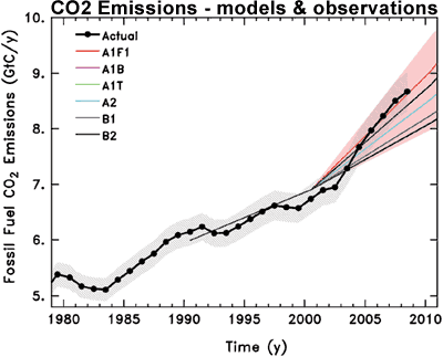
Figure 3: Observed global CO2 emissions from fossil fuel burning and cement production compared with IPCC emissions scenarios. The coloured area covers all scenarios used to project climate change by the IPCC (Copenhagen Diagnosis).

What Lies Ahead

So if we continue in a business-as-usual scenario, we should expect to see atmospheric CO2 levels accelerate rapidly enough to more than offset the logarithmic relationship with temperature, and cause the surface temperature warming to accelerate as well.  Monckton's claim of a "straight line" increase in global temperature ignores that in his preferred 'business as usual' scenario, we are currently on pace to double the current atmospheric CO2 concentration (390 to 780 ppmv) within the next 60 to 80 years, and we have not yet even come close to doubling the pre-industrial concentration (280 ppmv) in the past 150 years.  Thus the exponential increase in CO2 will outpace its logarithmic relationship with surface temperature, causing global warming to accelerate unless we take serious steps to reduce greenhouse gas emissions.  In fact, to continue the current rate of warming over the 21st Century, we would need to achieve IPCC scenario B1 - a major move away from fossil fuels toward alternative and renewable energy.

As for what amount of global warming is "harmless" and "dangerous" we will examine this question later on in another upcoming Monckton Myth.

0 0

Printable Version  |  Link to this page

Comments

1  2  Next

Comments 1 to 50 out of 86:

  1. I always knew there was something fishy about the figures Monckton tosses around. Now if only we could state the rebuttal as succinctly as Monckton stated the disinformation.
    0 0
  2. MattJ #1 - the problem is that it's very easy to make a false, unsubstantiated statement. It takes a lot more work to prove the statement is false. Monckton constantly takes advantage of this principle, which is why we have to have an entire series of Monckton Myths.
    0 0
  3. err yes - very thorough! that last paragraph is a bit of a brain twister. well it all is, but you cant give any wiggle room with these people. tamino has been examining 'noisy short-term temperature data', nice tidy up here http://tamino.wordpress.com/2011/01/06/sharper-focus/
    0 0
  4. Monckton must have learned his tricks from Fred Seitz, but then didn't they all (Seitz was considered the granddaddy of global warming skeptics). It's just the age old trick of casting doubt; usually with an ulterior motive/incentive. I don't know about you but I wouldn't walk a mile for a "Camel". And I wouldn't listen to anyone who casts doubt on an issue which is being put under the microscope by so many different scientific disciples that have provided substantial proof to the contrary. That's not to say that there isn't room for constructive criticism, and that's why blogs like this and RealClimate and others serve a very useful purpose in informing the public, which is refreshing in comparison to those blogs that more resemble the chaotic nature of a scrum.
    0 0
  5. Notice how he switches time periods in mid-paragraph, going from "since 1970" to "since 2001." It's like he consciously knows that focusing on the last decade alone will give a skewed picture of the temperature trend. I suspect the same is true of those who claim, "no warming since 1998!" It's hard to be convinced they can make these mistakes honestly. It's especially frustrating since Monckton repeatedly accuses Steketee of cherry-picking time periods or extreme weather events. Unfortunately, Monckton is increasingly adroit when it comes to the Gish Gallop. Usually the only two ways to deal with this are not to dignify the low-flying bull with a debate, or to write a book-length rebuttal. Sadly the former option isn't available in this case, especially since Monckton is a favorite for legislative testimony.
    0 0
  6. Monckton's problem was that Steketee said "in the last 40 years", forcing Monckton to start in 1970. This excludes UAH, which started in 1979, yet Monckton cited the UAH trend (roughly 1.3°C per century) anyway. It's bad enough to cherrypick UAH, but even worse to cherrypick it over a timeframe during 25% of which it didn't even exist! 2001 seems to be surpassing 1998 as the 'skeptics' preferred cherrypicked starting point. No doubt because the longer the timeframe, the clearer the warming signal. This creates a bit of a conflict though, because UAH has one of the largest warming trends since 2001 of any temperature data set. It's difficult to cherrypick when your preferred cherries keep changing. I picture Monckton hopping from one branch of the cherry tree to the next.
    0 0
  7. The sad thing is that virtually nobody in Monckton's "audience" has the attention span or the desire to check if what he says has any kernel of truth in it. They wouldn't read half way through a paragraph of this post without bursting with foam at the mouth. They like what he says. They enjoy hearing him talk. It speaks deeply to the emotional attachement they have for whatever ideology makes it unacceptable to them to take any action against CO2 emissions. No facts, graphs, references, observations can counter that. They're humans, they will go in the direction their emotions push them. Everything else is just rationalization. Very low quality rationalization with Monckton for sure, but only from the factual point of view. From the emotional point of view it is quite good, and that's all it takes for his audience. Nonetheless, the work done in this post is great for that part of the population that would actually check on his ramblings.
    0 0
  8. The problem is the facts so far disagree with this article. The Mona Loa data shows the increase in CO2 to be approximately linear so far. ftp://ftp.cmdl.noaa.gov/ccg/co2/trends/co2_annmean_mlo.txt Here is a graph of it with trend line. http://www.woodfortrees.org/plot/esrl-co2/from:1958/to:2010/plot/esrl-co2/from:1958/to:2010/trend #Least squares trend line; slope = 1.43127 per year There is no hint of substantial exponential increase but just to be sure I did a 2nd order fit in Excel It got the following function: y = 0.0122x2 + 0.8138x + 311.64 If you substitute 90 years for X you get 483.702 This is more than the 128.79 + 313.26 = 442.05 of the linear trend but since the effect is logarithmic the effect is a very slow increase. Log[b10] of 442.05 = 2.645 Log[b10] of 483.70 = 2.684 That is an increase in effect of 1.4 % more. So far the geometric increase isn't happening.
    0 0
  9. NETDR - are you joking? The trend is so obviously exponential in your own plot!
    0 0
  10. By the way, tamino addressed this question long ago. http://tamino.wordpress.com/2010/04/12/monckey-business/
    0 0
  11. Dana Did you understand my post ? The 2nd order equation is : y = 0.0122x2 + 0.8138x + 311.64 The supposed exponential growth is unimportant if the exponent is very very small as it is. [.0122] The difference in effect from a linear trend is trivial. 1.4 % in 90 years. Read the post again and tell me exactly where my "error" is.
    0 0
    Moderator Response: [Daniel Bailey] Read the Tamino post located at the link dana1981 provided you with. You'll find your answer there.
  12. Moderator "Read the Tamino post located at the link dana1981 provided you with. You'll find your answer there." I read the link but believe my analysis is better. I did a 2 nd order curve fit and he didn't. Also he didn't calculate the logarithmic effect which is vital to understand the effect. Tamano is welcome to his opinion but I disagree and the facts back me up.
    0 0
    Moderator Response: [Daniel Bailey] If you want us to take you seriously you'll have to do better than that. Tamino is a professional time-series analyst who has proven his worth in the climate blogging wars over the years. Dismissive handwaving of his work costs you dearly in the credibility department here. A proper way forward would be for you to publish your work in a peer-reviewed body, as Tamino has done in the past. And in the spirit of teaching the teacher, you could post your claims at Tamino's place, Open Mind.
  13. NETDR, in your formula 0.122 is a constant, not the exponent. The exponent is 2. And the logarithmic effect, as discussed in my article, is between forcing/temperature and CO2. The logarithmic effect has nothing to do with the (exponential) rate of growth of atmospheric CO2. You seem to be in way over your head here. To quote from tamino, who did a much, much more thorough analysis than you (emphasis added):
    "Over time, the growth of CO2 has NOT been linear, but it also has NOT been exponential. It’s been faster than exponential (as the logarithm has grown faster-than-linear, i.e., it has accelerated). And yes, the acceleration of log(CO2) (the faster-than-exponential growth of CO2) is statistically significant. That settles it."
    0 0
  14. Actually, I think NETDR has stumbled onto something, despite his lack of understanding of fitting and statistics. I suggest people go and grab the 30 day demo of TableCurve2D. A simple quadratic is a remarkably good fit to the data, with an adjusted Rsq of 0.9991. Other more complex equations fit the data better, but at the expense of any physical meaning.
    0 0
  15. Maybe NETDR & Chemware are talking at past Dana1981? A quadratic fit to the CO2 data is just that - no particular physical meaning. NETDR didn't calculate an appropriate logarithmic effect - his/her calculations do not assess exponential behaviour. Exponential behaviour is equivalent to log(CO2) being a linear function, for which Tamino in Monckey Business illustrates is slower than the actual growth of CO2 - which dana1981 links to and quotes above. The facts do not back up NETDR!
    0 0
  16. The Mona Loa data shows the increase in CO2 to be approximately linear so far.
    A very short section of a curve is also 'approximately linear', but it isn't, 'actually'. As pointed out above, the non-linearity of CO2 increase is evident from the linear trend superimposed in your own graph. Do you agree, NEDT, that the exponent is 2, rather than 0.122?
    0 0
  17. I agree with Phillippe #7. Deniers deny for emotional reasons, and ethereal stuff like data do not reach them. The sad part is that their shortsight is caused by an attachment to stuff that is threatened by the very AGW they don't want to see. A new world of changing climate will be a major enemy of free market, business-as-usual or individual freedoms
    0 0
  18. @15 Ian Love: Actually, a quadratic can have physical meaning as a second order Taylor expansion of a more complex function. In this instance, the rising atmospheric [CO2] is a function of economic activity and CO2 sequestration mechanisms. Economic + physical chemistry modeling, anyone ? I'm not at work right right now, but I'll have another play tomorrow with TC2D - I'm intrigued to see which simple equations best describe the data.
    0 0
  19. @chemware - looking to see what simple equations fit a finite sample of data best tells you next to nothing about the process that generates the data. For example, as you point out, a quadratic is a Taylor series expansion of a more complex (or simpler) function, so if a quadratic fits well, it may simply be because it is approximating an exponential. If a more flexible quadratic fits better than an exponential, it may simply be that the quadratic is better able to model the random variability in the data, than the less flexible exponential, and hence the difference in fit is meaningless as it is down to random chance (this is known as "over-fitting" in statistics). You don't need economic modelling to make inferences about emissions, as good records of emissions are kept (by e.g. the Carbon Dioxide Information and Analysis Center). The fact that the airborne fraction (the proporion of anthropognic emissions that accumulate in the atmosphere) is approximately constant, gives support from physical modelleling that emissions are rising approximately exponentially (I have done the differential equations myself to check that this is the case). The test Tamino uses to establish that the rise is faster than exponetial is unequivocal. If it were merely exponential, then taking logs should give a straight line; the fact that the resulting line curves upwards is definitive proof that the rise is faster than exponential. This remains true regardless of whether a quadratic or any other function provides a better least-squares fit.
    0 0
  20. You don't need anything other than a simple spreadsheet to check the Mauna Loa data. Check the residuals from the linear fit: if they're random then there's no acceleration. They're not, so there is. You can plot the data logarithmically like Tamino did (I did it for annual, rather than 10-yr means). And the annual data residuals show acceleration above exponential! (although we should be careful with individual periods - 1990 saw the USSR collapse for example) You test for the acceleration in a standard way (trend in the residuals) and you find it. You test it against an exponential increase too and you find an acceleration there.
    0 0
  21. Perhaps this would be worth a short post? You can estimate final CO2 from current trends, assuming we continue as usual. First I tested to see whether quadratic was a good fit. It's ok: you can test for acceleration by assuming C=At^2 where C is carbon, t time and A constant. Rearrange to get C^(1/2)=At. Not plot the two together and if the risiduals (difference between a straight line and the actual results) are not random then you have some kind of acceleration. In this case there is an acceleration and it's positive: we are increasing faster than with the square of time. We can use this to put a MINIMUM on the amount of CO2 we expect by 2100 assuming we continue on as Mauna Loa data says we have for the past 50 years or so. Take the annual differences in CO2 and then plot them against year then fit a line: the trend is the acceleration in change of CO2 per year per year. It is 0.026 +/- 0.04. You can assume a constant acceleration (i.e a quadratic) which we know is a MINIMUM for the CO2 changes we expect. Then you can use a SUVAT to determine final CO2: s = ut + (1/2)at^2 Where u is the current rate of increase of CO2, about 2ppm/yr averaged from 2001-10. a is the acceleration, or the 0.026 we just worked out. Therefore final s, or CO2 concentration in 90 years time at 2100 is just over 680 ppmv. (This is LOWER than the actual better fit) So we expect an additional minimum of 3 W m^-2 of CO2 radiative forcing in the next 90 years from the Mauna Loa data. On top of the ~1.8 W m^-2 from the past 160 years. Obviously an acceleration if you bother to look at the Mauna Loa data. Which Monckton doesn't. His analysis is simply wrong too: exp * ln is only linear in special cases. I did this in a rush literally on the back of an envelope and excel. Off to lunch, but I'll check it later. Please correct me if I got it wrong!
    0 0
  22. First of all I was incorrect the exponent is 2. [I saw it after I hit "submit"!] We don't need to assume a constant acceleration. The 3 rd order equation for a best fit is: y = -5E-05x3 + 0.0159x2 + 0.7345x + 312 So the rate of acceleration term is tiny. The sample is over 50 years so any acceleration should be evident. I am only looking at 90 years because we will have transferred to renewable fuel by then. Mark R said "You test for the acceleration in a standard way (trend in the residuals) and you find it. You test it against an exponential increase too and you find an acceleration there. " I like the third order polynomial better. I also took the log of the CO2 data and plotted it. The slope was .0018. The equation is: y = 0.0018x + 2.4878 Over a 90 year period the rate of increase in effect is almost negligible. You could do the increase in increase forever and the effect is negligible.
    0 0
  23. I think the central problem in Monckton's claim of "log(exponential) = linear" has perhaps not quite been addressed here... The reason people think of our growth in emissions as roughly exponential is that really is the standard assumption of economics - a roughly constant growth rate from year to year. That translates into a close to exponential rise in CO2 emissions, assuming carbon intensity doesn't change (or changes itself at an exponential rate) with a doubling time of around 30 years (say 2%/year growth). But the *total* CO2 concentration in the atmosphere is a combination of the *pre-industrial* value (280 ppm) plus this exponentially growing anthropogenic piece - i.e. something like: CO2(year) = 270 ppm + 100 ppm * 2^((year - 2000)/30) In the long run, that expression is going to be dominated by the exponential term. But for the next 50 years or so it's a *SUM* of a flat term plus an exponential. And the logarithm of that is not something that rises linearly, but something that rises faster than linear (for now).
    0 0
  24. @NETDR "So the rate of acceleration term is tiny." That is irrelevant; if the rise in CO2 is exponential (or faster) then the increase in radiative forcing will be (super-) linear, regardless of the acceleration. The log of an exponential is a linear function, it is a fact of mathematics that can't be circumvented by fitting polynomials. I think part of the problem is that there is a colloquial meaning of "exponential" used in hyperbolic statements about uncontrollable runaway growth. There is another mathematical definition. In this case, it is the latter that is relevant, but some are using the "hyperbolic" definition and hence are surprised that the deviation from a linear model is not that large. However, to the more mathematically inclined, that is no big surprise.
    0 0
  25. All, This is one of the fallacious statements made by Monckton: "CO2 concentration is rising in a straight line at just 2 ppmv/year at present and, even if it were to accelerate to an exponential rate of increase, the corresponding temperature increase would be expected to rise merely in a straight line." That first claim has been shown to be demonstrably false. The second claim is a "what if", but in the real world the appropriate mathematical and statistical treatment of the data (and appropriate nomenclature, as noted by Dikram @24) show that the we are already there. This really is a no brainer and it is disturbing that people are willing to go out on a limb and shred their own credibility by trying to defend Monckton's fallacies.
    0 0
  26. Dikran As is commonly accepted the log of the CO2 is proportional to the effect of the CO2. The log is increasing so slowly that the effect increases slowly too. Saying something is exponential is just hand waving if the exponential part is very low, which it is. Since the slope of the effect [log] is .0018 the increase is small. in 90 years the effect increases 16 %. The effect of the second derivative as shown above is negligible and is negative . [-5E-05x3 ]
    0 0
  27. NETDR, you're still doing the analysis wrong. You don't fit a curve to the log data. If the log data is linear then the growth is exponential. If the log data has grown faster than linearly (as is the case for the CO2 data), then the growth is faster than exponential. Tamino has already shown all of this. You're just doing the analysis wrong and thus arriving at the wrong conclusions.
    0 0
  28. Dana1981: "It's bad enough to cherrypick UAH, but even worse to cherrypick it over a timeframe during 25% of which it didn't even exist!" Speaking of cherry-picking UAH, I've noticed that over the same time period as the RSS, UAH trends significantly lower (though still upwards). I don't know why that is and it'd be presumptuous of me to speculate, but it seems to make UAH more attractive as a source for the obfuscation of temperature trends.
    0 0
  29. NETDR@26 The log of an exponential function is a linear function, regardless of what the "acceleration" is. Say we have an exponential function f(x) = A*exp{B*x} The second derivative (or acceleration is) f''(x) = A*B^2exp(B*x) Note the "acceleration" depends on the constants A and B. Now if we compute the log of f(x) we get g(x) = log(f(x)) = log{A} + B*x which is a linear function, whatever the values of A and B, and hence whatever the acceleration (which depends on A and B). I hope we agree so far. Now the radiative forcing due to CO2 is a logarithmic function of atmospheric concentration Forcing = C*log(f(x)) = C*log{A} + C*B*x This is also a linear function, but the slope depends on the rate constant of the exponential (B), but it also depends on the constant C which represents climate sensitivity. Thus whether the acceleration in the growth of CO2 is important depends on climate sensitivity, so you can't just dismis it without mentioning climate sensitivity. I appologise if making the argument in such basic mathematical terms appears condescending, but I couldn't think of any other way of demonstrating the flaw in your argument.
    0 0
  30. NETDR i've tried to reproduce your data but i couldn't. I was able to reproduce only the same linear trend when using alog10 of concentration instead of the natural logarithm, but a different offset. Could you please give more details on what you did? By the way, using the correct logarithm I was able to reproduce Tamino's results (no surprise here); I can confirm that the coefficient of the quadratic term is statistically significant. Definitely CO2 is rising faster than exponential, let alone linearly.
    0 0
  31. NETDR: "I am only looking at 90 years because we will have transferred to renewable fuel by then" If there is no problem with continuing to pump CO2 into the atmosphere at the current, accelertaing rate, why would we switch to renewables?
    0 0
  32. @NETDR: it would have been simpler if you were capable of admitting when you're wrong. Here is another version of the graph you linked to. The long-term and short-term trends have been offset to be more visible. It is clear, looking at the short-term trends, that the rate is accelerating.
    0 0
  33. @19 Dikran Marsupial: OK, have had time to have a play, and here are the results with "simple" equations:
    RankRsqDOF Adj RsqStd ErrorF-statisticEquation
    10.99958380.99953850.47308052.822e+04Quartic(a,b,c,d,e)
    20.99939020.99933830.56663072.622e+04Cubic(a,b,c,d)
    30.99937500.99933590.56777843.917e+04Quadratic(a,b,c)
    40.99210750.99143582.03850482011.2298Exponent4(a,b,c,d)
    50.98904980.98836542.37649812212.8954Exponent3(a,b,c)
    60.98740940.98689552.52268083921.2121Line(a,b)
    I have ignored monster equations like 10th order Chebyshev's and Fourier polynomials. Both 3 and 4-parameter exponentials: y = A0 + A1*Exp(A2*(X+A3)) ) are a poor fit, both visually and statistically. Monckton's beloved straight line is very poor. Using the calibrated eyeball™, it is impossible to tell the difference between the three polynomials. Tamino's log plot simply tells us that it's not an exponential rise in [CO2] - which this comparison confirms. I would suggest you have a play with TC2D: it is quite surprising how well a quadratic fits the data, especially given the limited degrees of freedom of a quadratic.
    0 0
  34. RE: 29 Dikran We need to keep an eye on Monckton's sleight of hand as well. If CO2 did grow exponentially (which it isn't, it's growing faster than exponentially, Monckton simply went for the biggest lie he could - 'linear', to try and distract people from actual analysis), such that C = A exp (Bt) Then radiative forcing would be F = 5.35 ln (C) = 5.35 ln (A exp(Bt) ) = 5.35 ( ln(A) + Bt ) So the radiative forcing increases linearly with time, but that does not have to mean that temperature increases linearly with time... Consider the case of a very quick change in temperature to illustrate. Change in temperature rate = dT/dt = (1/C) dQ/dt where C is the heat capacity. Let's say you raise dQ/dt linearly very quickly (over a period of weeks, say) such that the system doesn't have time to warm up fully. If the system doesn't warm, it can't dump the heat, so dT/dt increases linearly. i.e. the rate of warming increases linearly, which is equivalent to a quadratic function of temperature in time. This should help illustrate how easy it is to pack in sleights of hand to lie to people.
    0 0
  35. #34: "the rate of warming increases linearly, which is equivalent to a quadratic function of temperature in time." Exactly. Linear forcing equates to an increasing rate of temperature increase, which matches observation: see the graph attached to the comment here.
    0 0
  36. chemware@33 You are missing the point, fitting polynomials tells you next to nothing about the underlying process. Unless you properly account at the uncertainty in the model fit, it doesn't even tell you that the rise definitely isn't exponential (hint: compute the Bayes factor for the exponential model against the polynomial - d.o.f. is only a very coarse measure of the complexity of a model). The reason I wouldn't fit a polynomial is that it wouldn't tell me anything interesting about the data, qualitatively or quantitatively that I didn't already know from the exponential model fit. The key point is that emissions are rising faster than exponential, so assuming radiative forcing is a logarithmic function of atmospheric concentration then radiative forcing will be rising super-linearly (and hence Monckton's argument is clearly incorrect). It doesn't matter that the rise in CO2 is not exactly exponential, it depends on economic activity, so it is never going to be as simple as that, but is there any point in modelling the deviations from exponential caused by economic cycles etc.? I'd say "no", because (a) they have very little to do with climate and (b) the can't reliably be predicted.
    0 0
  37. I think it is a matter of semantics Something can be technically increasing at a geometric rate and the effect not be serious. [if the exponential term is small] Sounds scary though doesn’t it ? When all is said and done the effect of CO2 is Logarithmic. [Natural log] So if LN (CO2) is increasing at a serious rate there is a problem. If the rate of LN(CO2) is increasing but at a slow rate there is no problem. The next problem is the rate of increase of increase which I will discuss in detail below. Tamino’s paper says it is increasing too but he is coy about how much. The information is there if you dig for it. Increase of effect: I Googled the Mauna Loa data and put it into an Excel spreadsheet. And plotted the Natural log of the data. ftp://ftp.cmdl.noaa.gov/ccg/co2/trends/co2_annmean_mlo.txt The equation it [Excel] came up with was: y = 21.453Ln(x) + 282.77 Which plots as almost an asymptote. [Plot the above equation if you don’t believe me.] It increases but very slowly and each year the increase appears to be slower. You can also pull the raw data into Excel and check me. Increase of rate of increase: I read the Tamino paper and he is correct that the rate is increasing but so slowly that there is no problem. The effect [LN] of the change is going up slightly but only slightly. The amount looks scary but the actual effect isn’t. IF you take Tamino’s non peer reviewed posting and look at the rate of the increase he shows it is very slow. I redid the method he wrote about. [10 year periods, 1 year delay in start dates] I got very similar looking chart with CO2 increasing about 2 PPM/year in 2010. At a liner rate of increase that would mean it increased by 1 PPM in 50 years [because it started at about 1 ppm] or 2/100 PPM per year or 1.8 PPM in 90 years. That is pretty slow. I will discuss the rate of change of the rate of change below. The Ln of his chart is pretty flat meaning little increase in effect. He does take the LN of the delta and he blows up the scale to make it look scary but the actual effect is not scary at all. If you read the chart carefully the rate of growth of the Ln [the effect] is ..0055 per year in 2010 which is very slow. Since the Ln at that time is 5.965582 then .0055 increase is tiny. Technically the rate of increase [2 nd derivative] is increasing but so what ? In 300 years or so the increase in increase might become significant in 90 it isn’t ! Just saying it is increasing isn’t enough. Tamino’s whole paper just says certain things happen and doesn’t evaluate the effect of those things. If you believe in CAGW and don’t read it carefully it might be convincing [and scary] but under close analysis it isn’t scary at all. I know the intent of the article is to mock Lord Monckton but essentially he is right. The fact that the rate of increase went from 1 PPM to 2 PPM in 50 years has almost no real world implications. (It is a debating game gotcha though. ) Computing the 90 year effect of CO2 using a linear function results in a tiny error. Since the effect is logarithmic the real effect change between 1958 and 2010 is Ln(CO2 2010) – Ln (CO2-1958)/Ln(CO2-1958) = 4 % change in 52 years. Big deal ! So unless the nations of the world start emitting more CO2 and the rate of increase s increasing faster than it has so far there is no problem.
    0 0
    Moderator Response: [Daniel Bailey] Sure looks like a Thelma & Louise to me: Yup, no problem.
  38. Moderator Apparently CO2 has very little effect. The huge amount your graph shows has at most caused .7 ° C and even that amount is overstated since the records began during a little Ice age when the sun was dormant. About half of the .7 was caused by solar increase and positive feedbacks. Or do positive feedbacks only work with CO2 warming ?
    0 0
    Moderator Response: [Daniel Bailey] "Apparently CO2 has very little effect. Incorrect; see here. To address the rest of your misconceptions, use the search function in the upper left corner to find many posts addressing those issues.
  39. NETDR, I suggest you actually read the article I wrote. The IPCC models various emissions scenarios, and in the 'business as usual' scenario which I presume you advocate, the planet warms approximately 4°C between 2000 and 2100. You also repeat Monckton's error of ignoring the 'warming in the pipeline'. Basically you're just repeating all the mistakes Monckton made, which makes me think you either didn't read the article, or didn't process anything it said.
    0 0
  40. Also, about 80% of the warming over the past century is anthropogenic. Again, that doesn't account for the warming yet to come from the CO2 we've already emitted.
    0 0
  41. Dana The CO2 analysis Tamino and I did doesn't support the supposed rapid increase in the rate of CO2 emission which gloomy predictions are based. As I showed above the rate is just a little faster than linear. In 90 years it is just a few percent and the (Ln) effect is even less.
    0 0
  42. NETDR @41 The CO2 analysis Tamino and I did doesn't support the supposed rapid increase in the rate of CO2 emission which gloomy predictions are based. Take a look at the graph in the original article. Most "gloomy predictions" are based (in the worst case) on the A1FT emission scenario. It's obvious (again, just by eyeballing that graph) that CO2 emissions are growing even faster than that. Therefore, the "gloomy predictions" are (unfortunately) more than justified. Or am I missing something?
    0 0
  43. NETDR@41 "As I showed above the rate is just a little faster than linear. In 90 years it is just a few percent and the (Ln) effect is even less. " Which is entirely irrelevant. It is the slope of log(CO2) that is the immediate problem, not the curvature. log(co2) being linear means that the eventual equilibrium temperature of the planet is also rising linearly, at a rate determined by climate sensitivity (hence the three degrees per doubling of CO2). A linear log(CO2) is bad enough, worrying about a slight acceleration over linear is just rearranging the deck chairs on the titanic.
    0 0
  44. Dana The key word is eventually. The rate of CO2 buildup even including the acceleration is quite small. Some people think we have passed "peak oil" and we will have to convert to alternative fuels in the next 50 years. Their prices will come down and the conversion will be relatively painless. The warming in the pipeline argument is probably not true since the heat which is supposedly building up in the ocean isn't building up at all. See the "missing heat" argument which Trenberth seems to be losing. Even if the missing heat is hiding at the bottom of the ocean it isn't going to do much warming until it comes to the surface is it ?
    0 0
  45. NETDR @44, So rather than admitting you are wrong, the goal posts get shifted and a number of red herrings get trotted out. Sorry, that is not good enough, and to me suggests that you are not here to debate the science in good faith. Also, it seems that you are trying to squeeze in as much misinformation as you can in one post. Peak oil is not the primary concern, coal is-- we still have mountains of the stuff to mine and burn. "The warming in the pipeline argument is probably not true since the heat which is supposedly building up in the ocean isn't building up at all." Again, you need to back this up with some actual facts (and not some half-baked paper published in a dodgy journal by Knox and Douglass). For now, you have simply made an unsubstantiated assertion. "See the "missing heat" argument which Trenberth seems to be losing." Trenberth has not "lost" the heat. Just because one cannot find something because of incomplete data sampling, doesn't mean that it is not there. Maybe it is time to resurrect "DSCOVR (Deep Space Climate Observatory) that George Bush Jnr. scrapped. "Even if the missing heat is hiding at the bottom of the ocean it isn't going to do much warming until it comes to the surface is it?" Well, actually that may already be happening (see here), and it will most certainly be something for future generations to worry about.
    0 0
  46. #41: "As I showed above the rate is just a little faster than linear." Stunning. The annual rate of change at MLO is given here; for the past 5 years its been between 1.7 and 2.3 ppm/year. From 1970-1974 (also 5 years) it averaged 1.1 ppm/year. That means the rate of increase has nearly doubled in less than 40 years. This 'accelerating' or concave up behavior for CO2 as a function of time is critical, as it overwhelms the slightly concave down behavior of the log function. What you calculate when you take log CO2 is the forcing. Increasing forcing results in increasing rates of temperature change, as shown by Dikran Marsupial. Here's what you get with increasing forcing: --- from comment here. Those temperature anomaly curves increase in slope regardless of the sensitivity used (those shown are 0.6, 1.7 and 3 degrees C per doubling of CO2). So your attempt to minimize the impact of increasing atmospheric CO2 is utterly incorrect; as jhudsy says, the gloomy predictions are indeed fully justified.
    0 0
  47. I'm not going to argue with NETDR anymore, except to point out that his claim that ocean heat content is no longer building is false and was refuted in Monckton Myth #1. He's wrong, as will be obvious to anyone reading this comment thread. But he's clearly not willing or able to realize that he's wrong, so arguing with him further is a waste of time.
    0 0
  48. mouncounbter So from 1958 to 2010 [52] years the increase in CO2 has gone from 1 PPM per year to 2 PPM per year. Big deal. In the next 50 years if it goes from 2 PPM per year to 4 PPM per year that is a very small amount. The flattening effect of the LN function is very strong. A straight line increase rolls over to look like a horizontal asymptote as each molecule does less and less warming. The CO2 curve even with the minuscule rate increase is essentially a straight line [linear] function. Plot the values for the 52 year and see it is almost a horizontal asymptote. Plot it and see for yourself. Oh I forgot alarmists never plot anything or think for themselves do they ? Computing the 90 year effect of CO2 using a linear function results in a tiny error. Since the effect is logarithmic the real effect change between 1958 and 2010 was actually [Including the slight increase in rate] Ln(CO2-2010) – Ln (CO2-1958)/Ln(CO2-1958) = 4 % change in 52 years. Big deal ! Admit it this discussion is over and you lost.
    0 0
    Moderator Response: The original post is about Monckton's claim of linear warming. muoncounter showed you (again) the nonlinear warming caused by nonlinear increases in CO2. You keep saying the extra (more than linear) increases are not a problem, without addressing the actual problem of more than linear increases in warming. The difference of even "just" one more degree of warming on top of the linear warming is quite important in consequences. If you want to argue that is not important, type "It's not bad" in the Search field at the top left of the page.
  49. #48: "I forgot alarmists never plot anything" As you clearly missed it, the graph is in #46. As you clearly don't understand it, those blue deltaT curves are temperatures calculated from forcing functions based on natural log CO2 as a function of time. Since you clearly still don't understand what that means, here's an easy-to-read wiki link. The relevant lines begin with Delta TS = and Delta F = . The big triangle is 'Delta'. And since you clearly don't see the importance of any of this, those red dots are actual temperature anomalies (shifted to 0 in 1880). Sure looks like the red stuff is coming up between two of the blues, matching the rate of change pretty well. That's what's called a match of observation to model -- and it's a sign that the model is pretty good. Thank you for demonstrating so admirably the total failure of this denialist argument and the total abandonment of reality that is needed to cling to it. But I do agree with you, this discussion is over.
    0 0
  50. I can't seem to follow your math here NETDR, You seem to be saying that going from a linear(y = 1.43127x + 313.26) to a quadratic(y = 0.0122x^2 + 0.8138x + 311.64) only marginally changes the outcome. Yet if I run the numbers on the two i get significantly different results. Today CO2 (from mlo) is 389.78ppm, in 2100(90 years from now) your linear projects it to be 516.50ppm and your quadratic projects 673.20ppm, a 30% difference! Now the radiative forcing(as I understand it) is proportional to the ln of the change in the CO2(ie ∆F = 5.35*ln(C/Co)). If we take today as the baseline and look 90 years into the future there is a significant difference between the two. For your linear: ∆F = 5.35*ln(516.50/389.78) = 1.51 For your quadratic: ∆F = 5.35*ln(673.20/389.78) = 2.92 So If CO2 is raising at your quadratic rather than your linear then we should expect to see almost double the temperature rise over the next 90 years. To say that is a trivial difference just seems plain wrong to me.
    0 0

1  2  Next

You need to be logged in to post a comment. Login via the left margin or if you're new, register here.


The Consensus Project Website

THE ESCALATOR

(free to republish)


© Copyright 2024 John Cook
Home | Translations | About Us | Privacy | Contact Us