


 Arguments


Global warming and the El Niño Southern Oscillation
What the science says...
| Select a level... |
 Basic
Basic
|
 Intermediate
| |||
|
El Nino has no trend and so is not responsible for the trend of global warming. |
|||||
Climate Myth...
It's El Niño
"Three Australasian researchers have shown that natural forces are the dominant influence on climate, in a study just published in the highly-regarded Journal of Geophysical Research. According to this study little or none of the late 20th century global warming and cooling can be attributed to human activity. The close relationship between ENSO and global temperature, as described in the paper, leaves little room for any warming driven by human carbon dioxide emissions. The available data indicate that future global temperatures will continue to change primarily in response to ENSO cycling, volcanic activity and solar changes." (Climate Depot)
At a glance
This particular myth is distinguished by the online storm that it stirred up back in 2009. So what happened?
Three people got a paper published in the Journal of Geophysical Research. It was all about ENSO - the El Nino Southern Oscillation in the Pacific Ocean. ENSO has three modes, El Nino, neutral and La Nina. In El Nino, heat is transferred from the ocean to the atmosphere. In La Nina, the opposite happens. So within ENSO's different modes, energy is variously moved around through the planet's climate system, but heat is neither added nor subtracted from the whole. As such, in the long term, ENSO is climate-neutral but in the short term it makes a lot of noise.
The paper (link in further details) looked at aspects of ENSO and concluded that the oscillation is a "major contributor to variability and perhaps recent trends in global temperature". First point, sure. Second point, nope, if you accept climate trends are multidecadal things, which they are.
That might have been the end of it had the authors not gone full-megaphone on the media circuit, promoting the paper widely in a certain way. "No scientific justification exists for emissions regulation", they loudly crowed. "No global warming", the denizens of the echo-chamber automatically responded, all around the internet. This is how climate science denial works.
Conversely, the way that science itself works is that studies are submitted to journals, peer-reviewed, then some of them get published. Peer review is not infallible - some poor material can get through on occasion - but science is self-correcting. So other scientists active in that field will read the paper. They may either agree with its methods, data presentation and conclusions or they may disagree. If they disagree enough - such as finding a major error, they respond. That response goes to peer-review too and in this case that's exactly what happened. An error so fundamental was found that the response was published by the same journal. The error concerned one of the statistical methods that had been used, called linear detrending. If you apply this method to temperature data for six months of the Austral year from winter to summer (July-December), it cannot tell you that during that period there has been a seasonal warming trend. So what happens if you apply it to any other dataset? No warming! Bingo!
A response to the response, from the original authors, followed but was not accepted for publication, having failed peer-review. At this point, the authors of the rejected response-to-the-response started to screech, "CENSORSHIP" - and the usual blogosphere battles duly erupted.
It was not censorship. Dodgy statistical techniques were picked up by the paper's highly knowledgeable readership, some of whom joined forces to prepare a rebuttal that corrected the errors. The response of the original paper's authors to having their errors pointed out was so badly written that it was rejected. That's not censorship. It's about keeping garbage out of the scientific literature.
Quality control is what it's all about.
Please use this form to provide feedback about this new "At a glance" section. Read a more technical version below or dig deeper via the tabs above!
Further details
ENSO, the El Nino Southern Oscillation, is an irregular but well-understood phenomenon that affects the Eastern and Central Pacific Oceans. It is important both on a local and global basis, since it not only causes changes in sea-surface temperatures. It also affects the thermal profile of the ocean and both coastal and upwelling ocean currents.
Such changes can and do affect the diversity and abundance of important edible seafood species. Cold and warm-water forms are forced to migrate to where they find the conditions more to their liking. El Nino events in particular, where warm waters prevail close to the sea surface, can inflict a temporary loss of commercially important species of fish and squid from where they are traditionally fished. Some coastal communities along the Pacific seaboard of South America have a strong dependency on such fisheries. As such, prolonged El Nino conditions can be seriously problematic.
The warm El Nino mode of ENSO also affects global temperatures, as heat energy is transferred from ocean surface to the atmosphere. A strong El Nino is easily capable of raising temperatures above the upward slope that represents the change in radiative forcing caused by our increasingly vast greenhouse gas emissions - global warming, in other words. Conversely, the opposite to El Nino, La Nina, suppresses global temperatures. When several La Nina years occur in a row, climate science deniers are given the opportunity to insist that the world is cooling. This has happened before, most notably in the post-1998 period.
However, as fig. 1 shows, global temperature is rising independently of the short-term ENSO noise. Fig. 1 also shows that 2022 was the warmest La Nina year in the observational record. In fact, El Nino, La Nina and neutral years are all getting warmer.
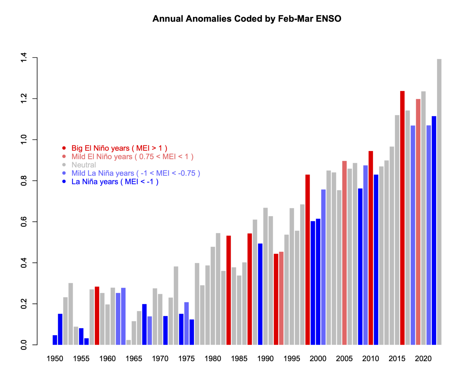
Fig. 1: variations in ENSO in a warming world. This plot therefore shows two independent phenomena that affect climate: the noisy ENSO and the underlying relentless upward climb in temperatures caused by our rapidly-increasing emissions of CO2 and other greenhouse gases. Temperature records typically get broken in El Nino years because the temperature is given an extra boost. 2016, a major El Nino year, held the global temperature record for a few years, but 2023 saw that record fall again. 2023 is in grey because that El Nino did not develop until later in the year. Graphic: Reaclimate.
The reader should by now be in no doubt about the difference between the long term global temperature trend caused by increased greenhouse gas forcing and the noise that shorter-term wobbles like ENSO provide. You would have seen something similar during the descents into and climbs out of ice-ages too. That's because ENSO has likely been with us for a very long time indeed. Ever since the Pacific Ocean came close to its present day geography, millions of years ago, it has likely been there.
The reader should by now be in no doubt about the difference between the long term global temperature trend caused by increased greenhouse gas forcing and the noise that shorter-term wobbles like ENSO provide. You would have seen something similar during the descents into and climbs out of ice-ages too. That's because ENSO has likely been with us for a very long time indeed. Ever since the Pacific Ocean came close to its present day geography, millions of years ago, it has likely been there.
Nevertheless, here we have something that warms the planet, even if that's on a temporary basis. As a consequence, some people with ulterior motives might just become interested. Over a decade ago now, that's what happened. A paper, 'Influence of the Southern Oscillation on tropospheric temperature' (Mclean et al. 2009) was published in the Journal of Geophysical Research. One of its co-authors, a well-known climate contrarian, commented:
"The close relationship between ENSO and global temperature, as described in the paper, leaves little room for any warming driven by human carbon dioxide emissions."
If you enter the above quote, complete with its quotation marks, into a search engine, you will get lots of exact matches. Strange? Not really, if you have studied the techniques of climate science denial.
- a paper is published that barely mentions global warming.
- its authors go on to distribute slogans implying that they have put yet another Final Nail in the global warming coffin.
- right-wing media of all sorts from newspapers to blogs ensure wide distribution of the talking-points.
- individuals serve to fill in the circulation-gaps.
This is how it works, time and again. However, glaring errors were soon noticed in the paper, leading a group of specialists to offer a rebuttal, published in the same journal a year later (Foster et al. 2010).
Statistics is not everyone's cup of tea, but a very straightforward explanation of the key error was provided by Stephen Lewandowsky, writing at ABC (archived):
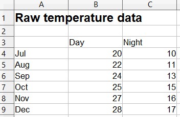
"This is best explained by an analogy involving daily temperature readings between, say, July and December anywhere in Australia. Suppose temperature is recorded twice daily, at midday and at midnight, for those 6 months. It is obvious what we would find: Most days would be hotter than nights and temperature would rise from winter to summer. Now suppose we change all monthly readings by subtracting them from those of the following month—we subtract July from August, August from September, and so on. This process is called "linear detrending" and it eliminates all equal increments. Days will still be hotter than nights, but the effects of season have been removed. No matter how hot it gets in summer, this detrended analysis would not and could not detect any linear change in monthly temperature."
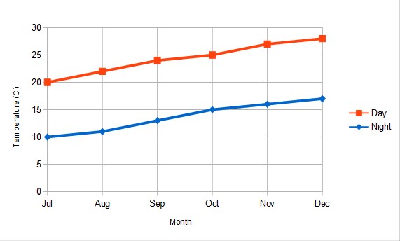
Anyone can do this in Excel. First input a series of representative temperatures for the transition from Austral winter into summer:
Reasonable? OK, then let's plot them. Still looks like what we'd expect. It gets warmer in Australia from July to December and nights are usually colder than days, right?
Now, let's do that detrending. This is what you get:
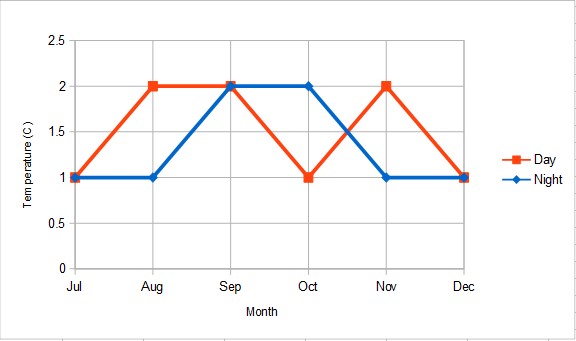
As Lewandowsky pointed out in his ABC article:
"Astonishingly, McLean and colleagues applied precisely this detrending to their temperature data. Their public statements are thus equivalent to denying the existence of summer and winter because days are hotter than nights."
In other words: Fail.
Last updated on 24 March 2024 by John Mason. View Archives


Sorry for the delay. I was responding to comments at other blogs and writing new blog posts.
skywatcher at 138 says: Bob, in all your focus on one region of the Earth, you have apparently neatly dodged important questions with relation to global warming and your unusual conjectures…”
Apparently, skywatcher, you’ve missed the fact that the discussion of sea surface temperatures was broken down into two parts of the global oceans, the East Pacific (90S-90N, 180W-80W) and the Rest-of-the-World (90S-90N, 80W-180). How is that “one region of the Earth”, skywalker? Sure looks like it covers the global oceans to me.
Also, are you aware that the warming of land surface air temperatures is primarily in response to the warming of the oceans, skywatcher? Refer to Compo and Sardeshmukh 2009: Oceanic influences on recent continental warming. The abstract reads:
That study was based on climate models by the way and you can get an idea of the order of magnitude using the ModelE Climate Simulations – Climate Simulations for 1880-2003 webpage, specifically Table 3.
And as I’ve shown, the satellite-era sea surface temperature and ocean heat content records do not confirm the existence of an anthropogenic warming component. Maybe you’ve missed this: the divergences during the La Niña events of 1988/89 and 1998-01 are when the Rest of the World data acquires its long-term trend. If the Rest-of-the-World sea surface temperature data cooled proportionally during the La Niña events of 1988/89 and 1998-2001, it would have no warming trend like the East Pacific!
skywatcher at 138 says: “1: Where's the heat coming from? The oceans, globally, are warming, the atmosphere is warming, and yet the Sun is not getting any brighter. What's your energy source?”
The sun is the primary energy source, but sea surface and ocean heat content warming can and do also take place without the exchange of heat, which is the result of teleconnections. The process through which the sun creates the warm water for El Niño events was described in my comment 139, where I replied to composer99:
El Niño and La Niña events are part of a coupled ocean-atmosphere process. Sea surface temperatures, trade winds, cloud cover, downward shortwave radiation (aka visible sunlight), ocean heat content, and subsurface ocean processes (upwelling, subsurface currents, thermocline depth, downwelling and upwelling Kelvin waves, etc.) all interact. They’re dependent on one another. During a La Nina, trade winds are stronger than normal. The stronger trade winds reduce cloud cover, which, in turn, allows more downward shortwave radiation to enter and warm the tropical Pacific.
If you’re having trouble with my explanation because it’s so simple, refer to Pavlakis et al (2008) paper “ENSO Surface Shortwave Radiation Forcing over the Tropical Pacific.” Note the inverse relationship between downward shortwave radiation and the sea surface temperature anomalies of the NINO3.4 region in their Figure 6. During El Niño events, warm water from the surface and below the surface of the West Pacific Warm Pool slosh east, so the sea surface temperatures of the NINO3.4 region warm, causing more evaporation and more clouds, which reduce downward shortwave radiation. During La Niña events, stronger trade winds cause more upwelling of cool water from below the surface of the eastern equatorial Pacific, so sea surface temperature to drop in the NINO3.4 region, in turn causing less evaporation. The stronger trade winds also push cloud cover farther to the west than normal. As a result of the reduced cloud cover, more downward shortwave radiation is allowed to enter and warm the tropical Pacific during La Niña events.
To complement that, here’s a graph to show the interrelationship between the sea surface temperature anomalies of the NINO3.4 region and cloud cover for the regions presented by Pavlakis et al.
That discussion explains why the long-term warming of the Ocean Heat Content for the tropical Pacific was caused by the 3-year La Nina events and the unusual 1995/96 La Niña. First, here’s a graph of tropical Pacific Ocean Heat Content. It’s color coded to isolate the data between and after the 3-year La Niña events of 1954-57, 1973-76 and 1998-2001. Those La Niña events are shown in red. Note how the ocean heat content there cools between the 3-year La Niña events. Anyone who understands ENSO would easily comprehend how and why that happens. It’s tough to claim that greenhouse gases have caused the warming of the tropical Pacific when the tropical Pacific cools for multidecadal periods between the 3-year La Niñas, Composer99.
As you can see, the warming that took place during the 1995/96 La Niña was freakish. Refer to McPhaden 1999 “Genesis and Evolution of the 1997-98 El Niño”.
McPhaden writes:
Based on the earlier description, that “build up of heat content” resulted from the interdependence of trade winds, cloud cover, downward shortwave radiation and ocean heat content. Simple. As you can see in the above graph, the upward spike caused by the 1995/96 La Niña skews the trend of the mid-cooling period, and if we eliminate the data associated with it and the 1997/98 El Niño, then the trend line for the mid-period falls into line with the others.
HHH
skywatcher, so La Niña events provide the naturally created fuel for El Niño events. More ENSO basics: An El Niño releases that heat, which is stored as warm water, from below the surface of the West Pacific Warm Pool. The warm water travels east and spreads across the surface of the eastern tropical Pacific. The El Niño releases heat through evaporation into the atmosphere, which is why tropical Pacific ocean heat content drops during an El Niño. Additionally, the convection, cloud cover and precipitation accompany that warm water east, sometimes almost halfway around the globe. These changes in location of the primary source of tropical Pacific convection and the resulting changes in atmospheric circulation, not a direct transfer of heat, are what cause surface temperatures to warm in areas remote to the eastern tropical Pacific.
Further to this, as I replied to doug_bostrom in my comment 103:
On the other hand, are you aware of teleconnections? Are you aware that there’s no heat transfer with teleconnections? Example: Why do the tropical North Atlantic sea surface temperature anomalies warm during an El Nino, doug? Do you know? There’s no direct exchange of heat yet the tropical North Atlantic warms during an El Niño. Why, doug? Could it have something to do with the slowing of the trade winds in the tropical North Atlantic in response to the El Niño? That would result in less evaporation, which is the primary way the oceans release heat. If there’s less evaporation, sea surface temperatures warm, do they not? Also, when the trade winds slow in the tropical North Atlantic in response to an El Niño, there’s less upwelling of cool waters from below the surface and less entrainment of that cool subsurface water. That would cause the seas surface temperatures to warm too.
HHH
If you don’t like my explanation, skywatcher, refer to Wang (2005) ENSO, Atlantic Climate Variability, And The Walker And Hadley Circulation for a more detailed discussion. And if you’d like a discussion of teleconnections for the rest of the world, refer to Trenberth et al (2002) Evolution of El Niño–Southern Oscillation and global atmospheric surface temperatures.
A quick note about Trenberth et al (2002). They qualify the results of their global warming attribution with:
The divergences between the Rest of the World data and the scaled NINO3.4 data during the 1988/89 and 1998-01 La Niña events are those ENSO residuals.
skywatcher at 138 says: “2: What's the physical mechanism involved, if it's not the rise in greenhouse gases? Sloshing water about the oceans does not appear adequate if the oceans, as a whole, are warming.”
Your representation of ENSO as “Sloshing water about the oceans” clearly indicates you lack a basic understanding of the topics being discussed. Please refer to my preceding reply to you for the answer to this question.
skywatcher at 138 says: “3: Why is this mechanism unidirectional, when ENSO is oscillatory?”
The impacts of ENSO are clearly not oscillatory. One look at the tropical Pacific OHC record clearly dismisses that idea. They would be better described as a discharge-recharge oscillator, where the recharge takes place during La Niña phases and the discharge takes place during El Niño. Also, the recharge varies, as can be seen in the response of the tropical Pacific Ocean Heat Content to the 1995/96 La Niña. I described above the recharge and discharge phases and the resulting teleconnections and confirmed it with data and with peer-reviewed papers. To further contradict your assertion that ENSO is oscillatory, with respect to sea surface temperatures, an El Niño releases warm water from below the surface of the west Pacific Warm Pool and the warm water spreads across the eastern tropical Pacific. That was the discharge phase. An El Niño does not consume the warm water. At the end of the El Niño, the warm water on the surface that’s left over from the El Niño is carried to the West Pacific and tropical East Indian Oceans, raising the surface temperatures there. The reverse does not occur during a La Niña. Further, there’s leftover warm water below the surface after the El Niño.
This leftover warm water was discussed in my reply to KevinC at 135:
The reasons for the divergences in the Rest-Of-the-World data during the 1988/89 and 1998-2001 La Niñas are physical, KevinC. You can try to eliminate or minimize them using models, but they exist. East Pacific El Niños like the 1986/87/88 and 1997/98 El Niños release vast amounts of warm water from below the surface of the west Pacific Warm Pool. Much of that warm water spreads across the surface of the central and eastern tropical Pacific. For the East Pacific El Niño events, like those in 1986/87/88 and 1997/98, that warm water impacts the surface all the way to the coast of the Americas (while with Central Pacific El Niño events it does not). The El Niños do not “consume” all of the warm water. At the conclusion of an El Niño, the trade winds push the leftover warm surface water back to the West Pacific. Additionally, there is left over warm water below the surface that’s returned to the west Pacific and into the East Indian Ocean via a Rossby wave or Rossby waves. This animation captures a Rossby wave returning warm water to the West Pacific and East Indian Oceans after the 1997/98 El Niño. Watch what happens when it hits Indonesia. It’s like there’s a secondary El Niño taking place in the Western Tropical Pacific and it’s happening during the La Niña. It’s difficult to miss it. (The full JPL animation is here.) Gravity causes that warm water to rise to the surface with time. The leftover warm water exists and it cannot be accounted for with a statistical model based on an ENSO index. You can see—you can watch it happen—the impacts of that warm water in this animation. There are no ENSO indices that account for the leftover warm water.
skywatcher at 138 says: “4: Assuming that a new unidirectional process must be a recent or temporary occurrence, otherwise we would have boiled or frozen awfuly quickly ... Why is your proposed physical mechanism a recent occurrence, when ENSO has been around for millennia, perhaps hundreds of thousands of years?”
The multiple assumptions are yours not mine and your assumptions are monumental. For example, we’ve got reasonable sea surface temperature-based ENSO records dating back to the opening of the Panama Canal in 1914. Can you prove ENSO did not have the same effect and cause the warming from about 1917 to 1944? I’ve limited my discussion to the satellite era of sea surface temperatures because the data is globally complete and it’s considered to be “the truth”. As I replied to Michael Sweet in my comment 133, which was a cut and paste from my book:
Refer to Smith and Reynolds (2004) Improved Extended Reconstruction of SST (1854-1997). It is about the Reynolds OI.v2 data we’ll be using as the primary source of data for this book:
The truth is a good thing, don’cha think?
skywatcher, as I’ve shown repeatedly throughout this exchange, the satellite-era sea surface temperature records and the ocean heat content data do not confirm the presence of an anthropogenic warming signal. You can believe what you want, but I refer to data, not climate models, for my understandings
skywatcher at 138 says: “5: Why is the well-understood mechanism of an enhanced greenhouse effect from long-lived GHGs not operating according to their physics, despite this physics neatly explaining both present climate and palaeoclimate changes?”
I’ll repeat my basic statement once more: the satellite-era sea surface temperature records and the ocean heat content records do not confirm the existence of an anthropogenic global warming component. And as I replied to KR at 134:
Downward longwave radiation appears to do nothing more cause a little more evaporation from the ocean surface, which makes perfect sense since it only penetrates the top few millimeters.
John Hartz says at 141: “You have not responded to the question I posed to you in #121. For everyone's convenience, I will repost it here… Do you believe the following graph to be a valid representation of Jan-Oct global land & and surface temperature anomalies with respect to the 1961-1990 base period for calendar years 1950 through 2012?”
The data in that graph appears to be an honest representation of the data, but would you like to explain what this has to do with a discussion about the long-term effects of ENSO?
To save you the time needed to scroll up, the following is what I wrote in an earlier comment to skywatcher:
Are you aware that the warming of land surface air temperatures are primarily in response to the warming of the oceans, skywatcher? Refer to Compo and Sardeshmukh 2009: Oceanic influences on recent continental warming. The abstract reads:
That study was based on climate models by the way and you can confirm the results at the ModelE Climate Simulations – Climate Simulations for 1880-2003 webpage, specifically Table 3.
HHH
And as I’ve shown, John, the satellite-era sea surface temperature and ocean heat content records do not confirm the existence of an anthropogenic component.
Could you have missed the importance of the divergences during the 1988/89 and 1998-01 La Niñas, John? The global oceans did not respond proportionally to the La Niña events of 1988/89 and 1998-01. That failure to cool proportionally during those La Ninas was why the sea surface temperatures for the Atlantic-Indian-West Pacific oceans (referred to as the Rest-of-the-World in earlier comments) acquired its long-term warming trend.
doug_bostrom says at 142: “Bob, where's the heat pump? How does it function?”
I don’t know how you’re defining heat pump, doug.
But I’ll cut and paste my earlier reply to skywatcher, as an explanation of ENSO to see if it agrees with how you’re defining heat pump. I wrote:
The process through which the sun creates the warm water for El Niño events was described in my comment 139, where I replied to composer99:
El Niño and La Niña events are part of a coupled ocean-atmosphere process. Sea surface temperatures, trade winds, cloud cover, downward shortwave radiation (aka visible sunlight), ocean heat content, and subsurface ocean processes (upwelling, subsurface currents, thermocline depth, downwelling and upwelling Kelvin waves, etc.) all interact. They’re dependent on one another. During a La Nina, trade winds are stronger than normal. The stronger trade winds reduce cloud cover, which, in turn, allows more downward shortwave radiation to enter and warm the tropical Pacific.
If you’re having trouble with my explanation because it’s so simple, refer to Pavlakis et al (2008) paper “ENSO Surface Shortwave Radiation Forcing over the Tropical Pacific.” Note the inverse relationship between downward shortwave radiation and the sea surface temperature anomalies of the NINO3.4 region in their Figure 6. During El Niño events, warm water from the surface and below the surface of the West Pacific Warm Pool slosh east, so the sea surface temperatures of the NINO3.4 region warm, causing more evaporation and more clouds, which reduce downward shortwave radiation. During La Niña events, stronger trade winds cause more upwelling of cool water from below the surface of the eastern equatorial Pacific, so sea surface temperature to drop in the NINO3.4 region, in turn causing less evaporation. The stronger trade winds also push cloud cover farther to the west than normal. As a result of the reduced cloud cover, more downward shortwave radiation is allowed to enter and warm the tropical Pacific during La Niña events.
To complement that, here’s a graph to show the interrelationship between the sea surface temperature anomalies of the NINO3.4 region and cloud cover for the regions presented by Pavlakis et al.
That discussion explains why the long-term warming of the Ocean Heat Content for the tropical Pacific was caused by the 3-year La Nina events and the unusual 1995/96 La Niña. First, here’s a graph of tropical Pacific Ocean Heat Content. It’s color coded to isolate the data between and after the 3-year La Niña events of 1954-57, 1973-76 and 1998-2001. Those La Niña events are shown in red. Note how the ocean heat content there cools between the 3-year La Niña events. Anyone who understands ENSO would easily comprehend how and why that happens. It’s tough to claim that greenhouse gases have caused the warming of the tropical Pacific when the tropical Pacific cools for multidecadal periods between the 3-year La Niñas, Composer99.
As you can see, the warming that took place during the 1995/96 La Niña was freakish. Refer to McPhaden 1999 “Genesis and Evolution of the 1997-98 El Niño”.
McPhaden writes:
Based on the earlier description, that “build up of heat content” resulted from the interdependence of trade winds, cloud cover, downward shortwave radiation and ocean heat content. Simple. As you can see in the above graph, the upward spike caused by the 1995/96 La Niña skews the trend of the mid-cooling period, and if we eliminate the data associated with it and the 1997/98 El Niño, then the trend line for the mid-period falls into line with the others.
HHH
skywatcher, so La Niña events provide the naturally created fuel for El Niño events. More ENSO basics: An El Niño releases that heat, which is stored as warm water, from below the surface of the West Pacific Warm Pool. The warm water travels east and spreads across the surface of the eastern tropical Pacific. The El Niño releases heat through evaporation into the atmosphere, which is why tropical Pacific ocean heat content drops during an El Niño. Additionally, the convection, cloud cover and precipitation accompany that warm water east, sometimes almost halfway around the globe. These changes in location of the primary source of tropical Pacific convection and the resulting changes in atmospheric circulation, not a direct transfer of heat, are what cause surface temperatures to warm in areas remote to the eastern tropical Pacific.
Further to this, as I replied to doug_bostrom in my comment 103:
On the other hand, are you aware of teleconnections? Are you aware that there’s no heat transfer with teleconnections? Example: Why do the tropical North Atlantic sea surface temperature anomalies warm during an El Nino, doug? Do you know? There’s no direct exchange of heat yet the tropical North Atlantic warms during an El Niño. Why, doug? Could it have something to do with the slowing of the trade winds in the tropical North Atlantic in response to the El Niño? That would result in less evaporation, which is the primary way the oceans release heat. If there’s less evaporation, sea surface temperatures warm, do they not? Also, when the trade winds slow in the tropical North Atlantic in response to an El Niño, there’s less upwelling of cool waters from below the surface and less entrainment of that cool subsurface water. That would cause the seas surface temperatures to warm too.
HHH
If you don’t like my explanation, skywatcher, refer to Wang (2005) ENSO, Atlantic Climate Variability, And The Walker And Hadley Circulation for a more detailed discussion. And if you’d like a discussion of teleconnections for the rest of the world, refer to Trenberth et al (2002) Evolution of El Niño–Southern Oscillation and global atmospheric surface temperatures.
A quick note about Trenberth et al (2002). They qualify the results of their global warming attribution with:
The divergences between the Rest of the World data and the scaled NINO3.4 data during the 1988/89 and 1998-01 La Niña events are those ENSO residuals.
HHH
Would you consider ENSO to be a heat pump, doug?
IanC says at 143: “So in short, you are very certain that you are correct, and see no possible reason for your analysis to be flawed? By the way, I'm mainly referring to PDO and decadal temperature trends.”
Is this a repeated question, IanC? If so, why are you asking it when I’ve already answered it? If not, then I’ll ask, which decadal temperature trends? Global? East Pacific? North Pacific? Pacific? If it’s the latter 3, I’ll repeat my earlier answer:
From my comment 103: As I noted earlier, the PDO does not represent the sea surface temperature of the North Pacific, the Pacific basin as a whole, or the East Pacific. Here’s a graph that compares the decadal variability of the PDO and the detrended and standardized sea surface temperature anomalies of the East Pacific, North Pacific (north of 20N, same as the PDO), and the Pacific as a whole:
http://i49.tinypic.com/slhb8y.jpg
Kevin C at 144: “You implicit model seems to be something like this: Ignoring volcanoes, the rest of the world temperatures track Nino34 with a single lag, except for some significant deviations which require another explanation.”
I’ve presented those explanations to you. You can watch them happen. Here’s my earlier reply:
The reasons for the divergences in the Rest-Of-the-World data during the 1988/89 and 1998-2001 La Niñas are physical, KevinC. You can try to eliminate or minimize them using models, but they exist. East Pacific El Niños like the 1986/87/88 and 1997/98 El Niños release vast amounts of warm water from below the surface of the west Pacific Warm Pool. Much of that warm water spreads across the surface of the central and eastern tropical Pacific. For the East Pacific El Niño events, like those in 1986/87/88 and 1997/98, that warm water impacts the surface all the way to the coast of the Americas (while with Central Pacific El Niño events it does not). The El Niños do not “consume” all of the warm water. At the conclusion of an El Niño, the trade winds push the leftover warm surface water back to the West Pacific. Additionally, there is left over warm water below the surface that’s returned to the west Pacific and into the East Indian Ocean via a Rossby wave or Rossby waves. This animation captures a Rossby wave returning warm water to the West Pacific and East Indian Oceans after the 1997/98 El Niño. Watch what happens when it hits Indonesia. It’s like there’s a secondary El Niño taking place in the Western Tropical Pacific and it’s happening during the La Niña. It’s difficult to miss it. (The full JPL animation is here.) Gravity causes that warm water to rise to the surface with time. The leftover warm water exists and it cannot be accounted for with a statistical model based on an ENSO index. You can see—you can watch it happen—the impacts of that warm water in this animation. There are no ENSO indices that account for the leftover warm water.
HHH
How does your model account for the leftover warm water, KevinC?
Same replies to KevinC at 149 and 152.
Bernard J. says at 145: “Specifically, I would like to know by exactly how much Tisdale believes that "[d]ownward longwave radiation" does or does not contribute to warming of the planet in terms of a particular DLR flux, and by what mechanisms that warming does - or indeed does not - does not occur.”
I believe this has been the underlying topic of discussion, Bernard J. The satellite-era sea surface temperature records and the ocean heat content records do not indicate that downward shortwave radiation has made any contribution to the warming.
Bernard J. says at 145: “Numbers and primary references would assist to make an objective and nuanced case.”
I’ll present the four datasets once again. For sea surface temperatures there’s the East Pacific Ocean and the Rest of the World data. In case you’ve missed this, the divergences during the La Niña events of 1988/89 and 1998-01 are when the Rest of the World data acquires its long-term trend. If the Rest-of-the-World sea surface temperature data cooled proportionally during the La Niña events of 1988/89 and 1998-2001, it would have no warming trend like the East Pacific! For ocean heat content, I presented as examples the Tropical Pacific and the North Pacific north of the tropics, both of which contradict the hypothesis of manmade greenhouse gas-driven global warming.
Tom Curtis at 146 says: “Why did Tisdale include a La Nina dominated period in his final period, when he must know that doing so will distort the comparison with the earlier period? And if La Nina dominated periods cause cooling, why has there been no cooling in the La Nina dominated period from Jan 1999 to the present?”
Tom, you’re referring to this graph. If you had been following the conversations on this thread you would have discovered that the global oceans did not respond proportionally to the La Niña events of 1988/89 and 1998-01 and that that failure to cool proportionally during those La Ninas was why the sea surface temperatures for the Atlantic-Indian-West Pacific oceans (referred to as the Rest-of-the-World in earlier comments) acquired its long-term warming trend. So why then are breaking the latest warming period at 1999 during the 1998-2001 La Nina when the Atlantic-Indian-West Pacific data acquires part of its long-term trend? If the Atlantic-Indian-West Pacific data cooled proportionally during the La Niña events of 1988/89 and 1998-2001, it would have no warming trend like the East Pacific!
Tom Curtis at 146 says: “Interestingly, in his comment @137 Tisdale quotes Compo and Sardeshmuk…”
You then go on, Tom, to attempt (and fail at your attempt) to fault me for using a single index in the above graph, but then immediately compromise your position by referring to your preferred single index, the Southern Oscillation Index.
Second, you’ve apparently misunderstood Compo and Sardeshmuk. Their discussion of a using a single index had to do with regression analysis. They wrote:
In this graph, I did not use the ENSO index in a regression analysis. I simply averaged the NINO3.4 sea surface temperature anomalies. There’s a very basic difference, Tom.
You also failed to recognize the importance of what I wrote after I quoted Compo and Sardeshmuk. It was:
Compo and Sardeshmuk are a step in the right direction, as I noted before I quoted them in my comment at 137.
Tom Curtis at 146 says: “Therefore simply taking the SST anomaly in the Nino 3.4 region over vastly different time periods cannot plausibly be considered a measure of ENSO activity. It in no way allows for the effects of other factors which we know will cause changes in the SST in the Nino 3.4 region as much as anywhere else.”
What “other factors” are referring to, Tom? Are you aware the authors of peer-reviewed papers about ENSO consider NINO3.4 sea surface temperature anomalies to be “a measure of ENSO activity”? An example is the Giese et al (2009) paper The 1918/19 El Niño. They argued that the 1918/19 portion of the 1918/19/20 El Niño was underestimated in the NINO3.4 sea surface temperature reconstructions, and that it was likely comparable in strength to the 1982/83 and 1997/98 El Niño events. Giese et al (2009) also suggested that the 1912/13 and 1939/40/41/42 El Niño events were also under-rated. If as you say, the NINO3.4 data “cannot plausibly be considered a measure of ENSO activity”, why would Giese et al (2009) have even written their paper, Tom? Why would NOAA use NINO3.4 data as the basis for its Ocean NINO Index? Why would Kevin Trenberth recommend NINO3.4 data over the SOI? Read on.
Please also note the dataset used by the ENSO experts who wrote that paper, Tom. It was HADISST, the same one I used. It was not HADSST3 or HADSST2, which you used in your comment 151.
With respect to your preference to the Southern Oscillation Index data, are you aware of all of the difficulties with that dataset? Refer to Trenberth (1997) The Definition of El Niño. He writes (my boldface):
It took a couple of years after that paper, but in response to those deficiencies in the SOI, Tom, NOAA and many scientists adopted NINO3.4 sea surface temperature anomalies and the Cold Tongue Index (which is based on sea surface temperature anomalies of a similar region) as the better measure of the frequency, magnitude and duration of El Niño and La Niña events.
Further to your comment 151: One of the reasons Giese et al used HADISST is because HADSST2 or HADSST3 are spatially incomplete. That is, there’s missing data. This can be seen in the output from the KNMI Climate Explorer of NINO3.4 data for the periods of 1912 through 1944 and 1944 through 1976, using a 15% cutoff as you did:
HADSST2 NINO3.4 from 1912-1944
HADSST2 NINO3.4 from 1944-1976
HADSST3 NINO3.4 from 1912-1944
HADSST3 NINO3.4 from 1944-1976
Note how much data is missing. I’ve limited the graphs to 3+ decade periods so that you could see all of the missing data, unlike your graphs in comment 151. That lack of data appears to have skewed the results you presented in comment 151, Tom.
If you had asked me what dataset I used in this graph, Tom, I would have told you HADISST. It’s been infilled so there’s no missing data. Here are the HADISST-based graphs from the KNMI Climate Explorer of NINO3.4 SST anomalies so you can visually compare them to the HADSST2- and HADSST3-based graphs above:
HADISST NINO3.4 from 1912-1944
HADISST NINO3.4 from 1944-1976
The differences between the HADISST-based NINO3.4 data and the others are quite extraordinary. Also if you had asked, I would have explained why I used HADISST—the HADSST2 and HADSST3 datasets are spatially incomplete in the NINO3.4 region. And I would have told you I used the base years of 1950-1979 in agreement with Trenberth (1997) The Definition of El Niño. He stated that 1950 to 1979 was the best base period for NINO3.4 sea surface temperature anomalies. Trenberth writes:
If you had asked, Tom, I would have been happy to explain all those things. You could have saved yourself a lot of time, and you would not have jumped to all the wrong conclusions.
Michael Sweet says at 147: “Your claim here that Gavin Schmidt at Realclimate says you can compare a single realization (what happened) to the model average and not to the model envelope is simply untrue.”
I don’t believe I claimed there “that Gavin Schmidt at Realclimate says you can compare a single realization (what happened) to the model average and not to the model envelope…”. I quoted Gavin Schmidt’s reply to the RealClimate comment at 30 Sep 2009 at 6:18 AM. It was:
Gavin said what he said. He was not talking about model-data comparisons; he was talking about model outputs in general, as was the quote I provided you from NCAR. NCAR wrote:
I’m NOT interested in the model noise, Michael; I’m also NOT interested in a “particular ensemble member where the initial conditions make a difference in your work”; I’m interested in the forced component that’s presented by the multi-model ensemble mean of all of the CMIP3 or CMIP5 climate models in my model-data comparisons, because it gives you “the best representation of a scenario”.
Note: The NCAR webpage I linked earlier seems to be offline, but the Wayback Machine has captured the text.