Climate Science Glossary

Term Lookup

Enter a term in the search box to find its definition.

Settings

Use the controls in the far right panel to increase or decrease the number of terms automatically displayed (or to completely turn that feature off).

Term Lookup

Settings


All IPCC definitions taken from Climate Change 2007: The Physical Science Basis. Working Group I Contribution to the Fourth Assessment Report of the Intergovernmental Panel on Climate Change, Annex I, Glossary, pp. 941-954. Cambridge University Press.

Home Arguments Software Resources Comments The Consensus Project Translations About Support

Twitter Facebook YouTube Mastodon MeWe

RSS Posts RSS Comments Email Subscribe


Climate's changed before
It's the sun
It's not bad
There is no consensus
It's cooling
Models are unreliable
Temp record is unreliable
Animals and plants can adapt
It hasn't warmed since 1998
Antarctica is gaining ice
View All Arguments...


Username
Password
New? Register here
Forgot your password?

Latest Posts

Archives

Lessons from Past Climate Predictions: IPCC SAR

Posted on 1 September 2011 by dana1981

The Intergovernmental Panel on Climate Change (IPCC) Second Assessment Report (SAR) was published in 1995, following the IPCC First Assessment Report (FAR), which we examined in the last Lessons from Past Climate Predictions entry.

In 1992, the IPCC published a supplementary report to the FAR, which utilized updated greenhouse gas emissions scenarios called "IS92" a through f.  The 1995 SAR continued the use of these emissions scenarios, and made the following statements about the state of climate models their future projections.

"The increasing realism of simulations of current and past climate by coupled atmosphere-ocean climate models has increased our confidence in their use for projection of future climate change. Important uncertainties remain, but these have been taken into account in the full range of projections of global mean temperature and sea level change."

"For the mid-range IPCC emission scenario, IS92a, assuming the "best estimate" value of climate sensitivity and including the effects of future increases in aerosol, models project an increase in global mean surface air temperature relative to 1990 of about 2°C by 2100. This estimate is approximately one third lower than the "best estimate" in 1990. This is due primarily to lower emission scenarios (particularly for CO, and the CFCs), the inclusion of the cooling effect of sulphate aerosols, and improvements in the treatment of the carbon cycle."

Aerosols

Perhaps one of the biggest improvements between the FAR and SAR was the increased understanding of and thus ability to model aerosols.  Section B.6 of the report discusses the subject.

"Aerosols in the atmosphere influence the radiation balance of the Earth in two ways: (i) by scattering and absorbing radiation - the direct effect, and (ii) by modifying the optical properties, amount and lifetime of clouds - the indirect effect. Although some aerosols, such as soot, tend to warm the surface, the net climatic effect of anthropogenic aerosols is believed to be a negative radiative forcing, tending to cool the surface"

"there have been several advances in understanding the impact of tropospheric aerosols on climate. These include: (i) new calculations of the spatial distribution of sulphate aerosol largely resulting from fossil fuel combustion and (ii) the first calculation of the spatial distribution of soot aerosol."

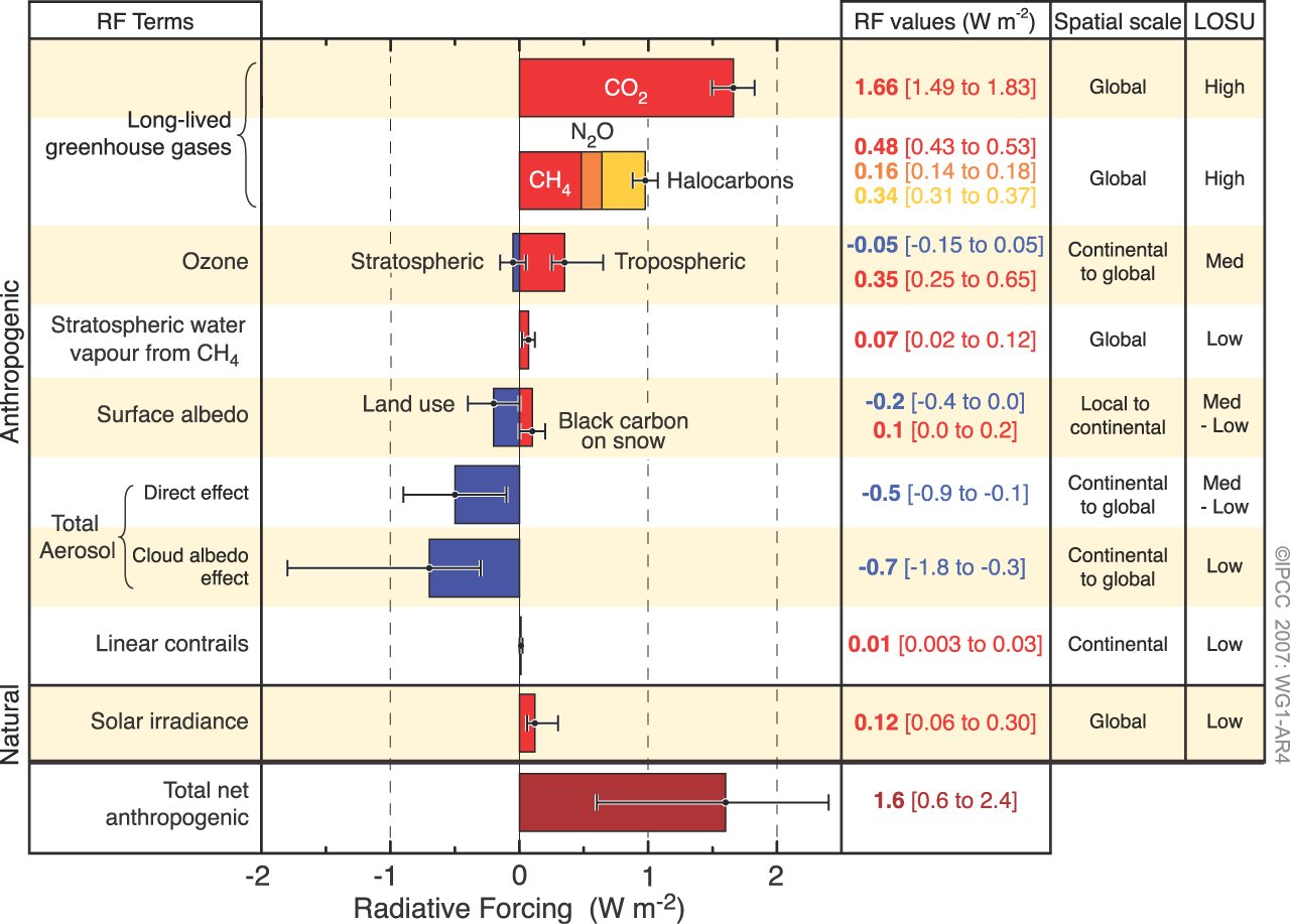
The SAR's estimated radiative forcings, including from aerosols, are shown in Figure 1.

SAR forcings

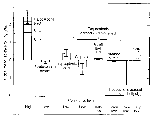
Figure 1: IPCC SAR etimates of the globally and annually averaged anthropogenic radiative forcing due to changes in concentrations of greenhouse gases and aerosols from pre-industrial times to 1992, and to natural changes in solar output from 1850 to 1992. The height of the rectangular bar indicates a mid-range estimate of the forcing whilst the error bars show an estimate of the uncertainty range.

Emissions Scenarios

The projected CO2 emissions and atmospheric concentrations in the IS92 scenarios are illustrated in Figure 2.

IS92 scenarios

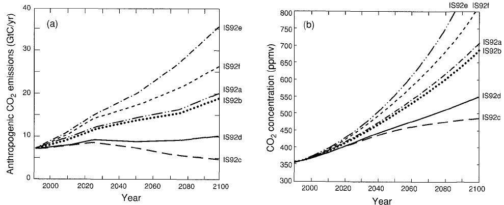
Figure 2: Total anthropogenic CO2 emissions under the IS92 emission scenarios and (b) the resulting atmospheric CO2 concentrations

So far, the IS92a and b scenarios have been closest to actual emissions, with scenarios e and f running just a bit high, and scenarios c and d increasingly diverging from actual emissions.  However, by the year 2011, the atmospheric CO2 concentrations in each scenario are not yet very different.  The IPCC SAR also provided a figure with the projected radiative forcings in Scenario IS92a (Figure 3).

IS92a projected forcings

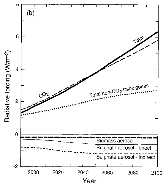
Figure 3: Projected radiative forcings in IPCC Scenario IS92a for 1990 to 2100.

One interesting aspect of this scenario is that the IPCC projected the aerosol forcings remaining strong throughout the 21st Century.  Given that aerosols have a short atmospheric lifetime of just 1 to 2 years, maintaining this forcing would require maintaining aerosol emissions throughout the 21st Century.  Since air quality and its impacts to human health are a related concern, it seems likely that human aerosol emissions will decline as the century progresses.  This issue was one significant change made in the IPCC Third Assessment Report (TAR) projections - the next entry in the Lessons from Past Climate Predictions series.

Global Warming Projections

The IPCC SAR also maintained the "best estimate" equilibrium climate sensitivity used in the FAR of 2.5°C for a doubling of atmospheric CO2.  Using that sensitivity, and the various IS92 emissions scenarios, the SAR projected the future average global surface temperature change to 2100 (Figure 4).

IPCC SAR Projections

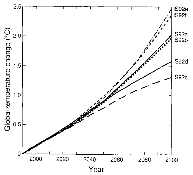
Figure 4: Projected global mean surface temperature changes from 1990 to 2100 for the full set of IS92 emission scenarios. A climate sensitivity of 2.5°C is assumed.

One helpful aspect of these scenarios is that the temperature projections from 1990 to 2011 are nearly identical, so the choice of scenarios makes little difference in evaluating the SAR projection accuracy to date.  So how do these projections stack up against observations?  We digitized the graph and compared it to observed temperatures from GISTEMP to find out (Figure 5).

SAR vs. observations

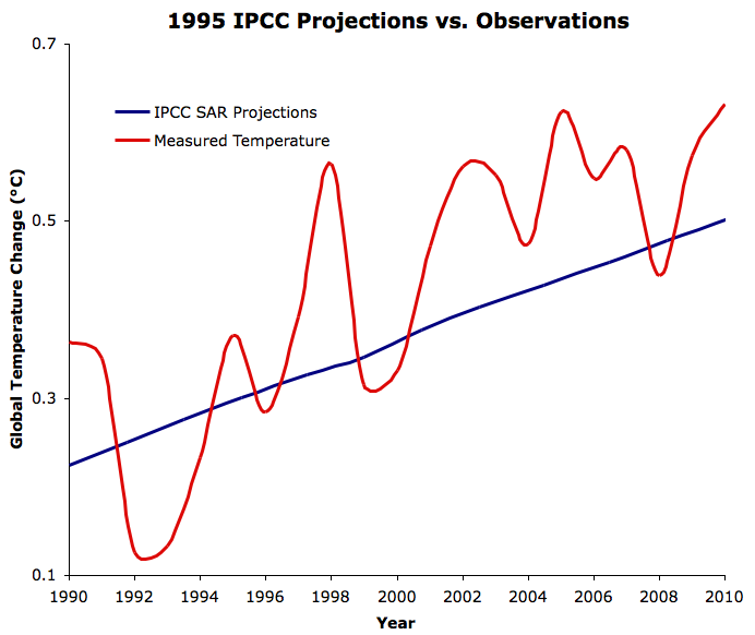
Figure 5: IPCC SAR global warming projections under the IS92 emissions scenarios from 1990 to 2010 (blue) vs. GISTEMP observations (red).

Actual Climate Sensitivity

As you can see, the IPCC SAR projections were quite a bit lower than GISTEMP's measurements, anticipating approximately 0.1°C less warming than was observed over the past two decades.  So where does the SAR projection go wrong?

The IS92a projected radiative forcings (Figure 3) have been quite close to reality thus far.  Updating the radiative forcings from the IPCC Fourth Assessment Report (AR4), the net forcing is almost the same as the CO2 forcing, which is close to 1.8 W/m2 in 2010.  This is almost exactly what the SAR projects in Figure 3.

However, the SAR used a radiative forcing of 4.37 W/m2 for a doubling of atmospheric CO2.  The IPCC TAR updated this value five years later with the value which is still in use today, 3.7 W/m2 (see TAR WGI Appendix 9.1).  Since the SAR overestimated the energy imbalance caused by a doubling of CO2, they also overestimated the climate sensitivity of their model.  If we correct for this error, the actual sensitivity of the SAR "best estimate" climate models was 2.12°C for doubled CO2, rather than their stated 2.5°C.

We can then compare the trend in the SAR model to the observed trend and determine what model sensitivity would have correctly projected the observed warming trend.  Matching the observations results in a model  equilibrium sensitivity of approximately 3°C (Figure 6).

SAR projections 3°C sensitivity

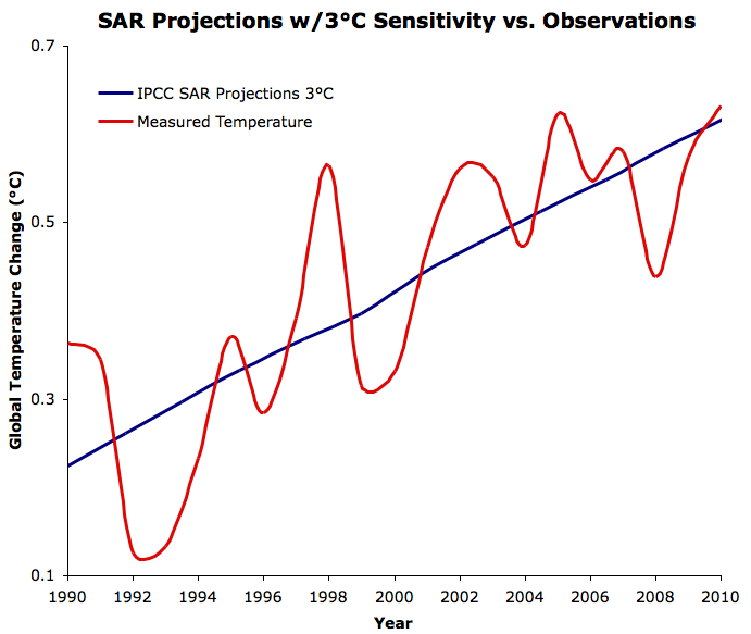
Figure 6: IPCC SAR global warming projections under the IS92 emissions scenarios from 1990 to 2010 with a 3°C equilibrium climate sensitivity (blue) vs. GISTEMP observations (red).

Learning from the SAR

The SAR projection of the warming over the past two decades hasn't been terribly accurate, although it was still much better than most "skeptic" predictions, because the IPCC models are based on solid fundamental physics.  The SAR accurately projected the ensuing radiative forcing changes, although it likely overestimated continued aerosol emissions in the second half of the 21st Century, and thus likely underestimated future warming.

The main problem in the SAR models and projections was the overestimate of the radiative forcing associated with doubling atmospheric CO2, and thus the underestimate of the equilibrium climate sensitivity to doubled CO2 (2.12°C).  In fact, the comparison between observations and the IPCC SAR projected warming provides yet another piece to the long list of evidence that equilibrium climate sensitivity (including only fast feedbacks) is approximately 3°C for doubled CO2.

0 0

Printable Version  |  Link to this page

Comments

Comments 1 to 31:

  1. What are the baselines for the lines in Fig 5 and 6? Figure 4, from the SAR starts with a reference point of 0 C in 1990. In Figure 5 and 6 you start at about 0.25C in 1990. What did you use for the offset baseline for the GISS data; and was the smooth a particular function or just a hand drawn approximation? Figures 4 and 5 are nice comparison graphs but what they are actually comparing is unclear.
    0 0
  2. Figures 5 and 6 use the GISTEMP baseline. The GISTEMP smoothing was done with the Excel "smooth" function. The Figure 5 caption explains what it's comparing.
    0 0
  3. By "Figures 5 and 6 use the GISTEMP baseline" I assume that you mean the 1951-1980 baseline, correct? There are many ways to adjust the baseline of the SAR projection to match the 1951-1980 baseline of the observed data. One method, which generates the best match between projection and observations is to wait until the end of the observation & projection period, and then go back and adjust the mean of the projection so it is equal to the actual observed mean temp over the projection period. It does appear that the 1990 SAR projection has been adjusted upward such that the mean projection matches the 0.424 C 1990-2010 mean of the GISS measured data. Is this what you did? Or is there some other calculation you used to change the 1990 SAR projection from the 0.00C shown in Figure 4, to the approximately 0.25C you show in Figures 5 and 6 ?
    0 0
  4. Charlie, there's no point in getting wrapped up in baselines. The baseline doesn't mean anything, it's just an arbitrary offset. All I did was offset the SAR projection in 1990 to match the GISTEMP 5-year running average value in 1990 (approximately 0.25°C). What matters are the temperature changes from 1990 to 2010, not the arbitrary baseline selection.
    0 0
  5. I agree that there is no need to get wrapped up in baselines, but it is also good practice to give basic information about what one is presenting. A simple "SAR projections have been offset such that the 1990 projection is equal to the GISS Temp 5 year running average in 1990" would have been sufficient, either in the main post, or in response to my question about baselines. (both the 1990 5 year running average and the 5 year gaussian smooth are 0.27 C, so your plot of projections is a bit low). ====================================== Since offsets or baselines don't matter, and the SAR projection is pretty much nothing but a straight line 1990-2010, then perhaps the most useful comparison would be simply to look at the 1990 to 2010 slopes. The SAR projection extended to 2100 is 1.5 C rise in 110 years, or 0.136 C / decade. The observed GISS land-sea global temp from 1990 through 2010 is 0.194 C/ decade. (per Excel linear regression Slope function). So the observed slope is 0.194/0.136 = 143% of projection. For the best match, we would simply increase the SAR projections by 43%. Treating the stated sensitivy of 2.5C/doubling as 2.12C, and then increasing that to 3 C/doubling is the equivalent of increasing the slope of the SAR projection by 3/2.12 = 42%. Not quite the perfect after-the-fact adjustment, but pretty close. So to summarize how we can show the excellent quality of the SAR projections, we simply need adjust the slope and offset of the the SAR projections to match the observed data. ============================== Regarding the F2x value ..... AR4 shows a range from 3.09 W/m2 for MIROC3.2(medres) up to 4.06 W/m2 for GISS-ER and GISS-EH. So the 3.7W/m2 is by no means the last word. The AR4 table equivalent to the TAR WGI Appendix 9 reference of the headpost is AR4 WG1 Chap 8, supplementary table S8.1. At the very end of (large pdf) AR4 WG1 Chap 8, supplementary info.
    0 0
  6. "So to summarize how we can show the excellent quality of the SAR projections, we simply need adjust the slope and offset of the the SAR projections to match the observed data."
    I didn't say the SAR projections were "excellent quality". In fact I basically said the opposite:
    "The SAR projection of the warming over the past two decades hasn't been terribly accurate"
    The purpose of adjusting the slope (sensitivity) and offset (baseline) is to see what model parameters would have made accurate projections, not to say the model and parameters were accurate.
    0 0
  7. However, the SAR used a radiative forcing of 4.37 W/m2 for a doubling of atmospheric CO2. The IPCC TAR updated this value five years later with the value which is still in use today, 3.7 W/m2 (see TAR WGI Appendix 9.1). Since the SAR overestimated the energy imbalance caused by a doubling of CO2, they also overestimated the climate sensitivity of their model. You appear to be saying that the SAR overestimated the climate sensitivity of their model and therefore underestimated the global temperature change. This is a bit counter intuitive. I'm sure that there is a perfectly good explanation but could you please elucidate for my benefit?
    0 0
  8. Sure Wombat, happy to. The relevant formula is dT = a*dF where dT is the change in temperature, a is the climate sensitivity parameter, and dF is the change in radiative forcing. In the SAR case, for dF = 4.37, they found dT = 2.5°C. So if we plug that into the formula: a = dT/dF = 2.5/4.37 = 0.57°C per W/m2 So for every 1 W/m2 forcing, the model results in 0.57°C warming. If we then use that climate sensitivity parameter to calculate what temperature change we would expect from the forcing associated with a doubling of CO2 (3.7 W/m2), we get: dT = 0.57 * 3.7 = 2.12°C What the SAR did was to overestimate how much of an energy imbalance is caused by a doubling of CO2. As a result, they also overestimated the temperature change in their model resulting from that doubling of CO2. And so they thought their model was more sensitive to CO2 doubling than it actually is. An important distinction is that they overestimated the model sensitivity specifically to doubled CO2, because they overestimated the forcing associated with doubled CO2. But the sensitivity parameter (0.57°C per W/m2) remains unchanged. Clear as mud?
    0 0
  9. Thanks dana
    0 0
  10. I think there is some circular reasoning here. Whatever model would gave a linear growth in temperature. Correcting those model for anything than actual CO2 curve compare to the real one is not a proof that the original model worked at all. For example, if the original model underestimated the temperature increase by a factor 2 and this could be traced back to a erroneous estimate of one constant, the model was wrong by a factor of two. That's it. Only correcting for CO2 curve make sense because this factor is unrelated to the physics of the model.Correcting for other factor that are directly related to the output of the model is another name for curve fitting, which will always work.
    0 0
  11. Yvan, see comment #6 and the conclusion of the post. Once again, I'm not saying the original model worked. I'm saying the original model would have worked with an equilibrium climate sensitivity of 3°C for 2xCO2. The SAR also ran models with sensitivities of 1.5°C and 4.5°C for 2xCO2 (though technically the sensitivities were 1.3°C and 3.8°C, for the reason discussed above). The former was much too low, and the latter was too high. Had they run a 3°C sensitivity model, it would have projected the correct amount of warming.
    0 0
  12. Dana- For my own preparedness I'm not clear on two things- The independent estimate of "A" the climate sensitivity factor. and why is this a linear equation? Off hand, given feed backs from changes in albedo as ice melts etc, would be non-linear, and as ice disppears from a region you lose the heat of melting. Or is that all taken into account in the construction of the radiative forcing? All definitional stuff I know... but I think clarity on the origin of the radiative forcing factor in current models might hep Yvan.
    0 0
  13. Dave123 - not sure what you mean about the independent estimate of the climate sensitivity. To your second question though, feedbacks are built into that sensitivity parameter. That's what "a" tells you - for a given radiative forcing, how much the temperature will change, including feedbacks.
    0 0
  14. Thanks for this Dana, have been trying to work out how to put all this into an explanation of how comparing models with observations gives us more understanding of the 3DegC sensitivity, The model update 2010 at RC also shows 3.3DegC sensitivity. appreciated.
    0 0
  15. Regarding linearity, I don't know of anything that is linear in the climate system, but, as any student of calculus knows, you can approximate any curve with line segments, and the shorter the segments, the less the error term. So, sure, I'd be very surprised if there were a constant (linear) relationship between CO2 and temperature over the range from slushball to ice-free states of the earth. However, given current orbital parameters and the positions, sizes, and shapes of the continents, and the current state of ice masses, it is possible to quantify a linear relationship that is good enough for the near future. WRT, "models are inaccurate", I think it was Gavin at RealClimate who pointed out that all you had to do to prove any model wrong was demand more accuracy out of it than the authors were able to code into it. That's the nature of models; all models are approximations. To be fair, you should compare the accuracy of models predicting warming as CO2 increases with models that don't. Shall we take a wild guess which set yields a better approximation of reality? Model factors are wrong, whatever. It's like a teacher (which in this case is history, not any of us) giving partial credit if the student shows their work on a long problem and the teacher is able to determine their answer world have been correct if they hadn't made a mistake at point X. If there are only one or two points, that somewhat validates the rest of the work. It's a little frustrating to see so many attacks on models because, AFAIK, all models with a halfway decent hindcasting ability predict continued warming under BAU. It doesn't really matter if we reach 4 degrees by 2100 or 2075; at some point we will cross a threshold beyond which the population can not be supported. It is going to continue to get warmer until we either switch to alternatives as our primary energy sources or society collapses.
    0 0
  16. My pleasure john. I also drafted up a post on the IPCC TAR which will be published in the near future. Matching the projections to observations yields a sensitivity of about 3.4°C for 2xCO2 there. Funny how we keep getting these same answers around 3°C, and yet the "skeptics" are certain sensitivity is somehow much lower than that. Either there's something very wrong with climate models, or something very wrong with Spencer and Lindzen et al.'s claims. Personally I'd put my money on the latter.
    0 0
  17. Chris G -
    "To be fair, you should compare the accuracy of models predicting warming as CO2 increases with models that don't."
    Actually we've done that. Click the button at the top of the post to see all our entries thus far in the 'Lessons from Past Climate Predictions' series. Easterbrook's cooling prediction is probably the most relevant. We also compared his prediction to Wallace Broecker's 1975 warming prediction in the Broecker post in the series. The purpose of this series is to fairly examine each warming or cooling prediction we can find and see where each went wrong and what we can learn from them. I'm also writing a book/booklet on the same subject.
    0 0
  18. Dana- Then A can't be constant with time, because feedbacks will be changing with time...albedo for example. The more ice we lose, the more land/ocean exposed, the more heat absorbed. Maybe I'm just confused on what is partioned into A and what into dF. My naive interpretation of dF has been the difference between solar irradiance and IR leaving the earth.
    0 0
  19. Oh, thanks Dana; I missed that. Looking... Really though, I wasn't targeting you, but rather the people who say things roughly like, your model is off by 0.2 C; therefore, all models are worthless.
    0 0
  20. What assumptions about the ozone hole in the atmosphere over Antarctica are embedded in the SAR model and forecasts?
    0 0
  21. Dave123 - there is a difference between short-term sensitivity, long-term fast feedback sensitivity, long-term sensitivity including slow feedbacks, etc. Maybe that's what you mean? James Wight had an excellent post discussing the various measures of sensitivity which I linked at the end of this post (click the "fast feedbacks" link in the last sentence). Chris G - I know, and I very much agree that people disrespect models way too much. No model is perfect, but there's almost always something we can learn from a model. One of the main points of this series is to see what we can learn from them. Learning from past model flaws is why models keep getting better and better. Badger - I'm not sure what assumptions they made about ozone depletion. Ozone plays a relatively minor role in the greenhouse effect though. But if you're interested, they probably talked about it in Chapter 6. You can download the whole SAR WGI report by clicking the first link in the post.
    0 0
  22. Dana- So sensitivity is something models calculate...rather than being an input into the model. I can't see a reason offhand why I would need sensitivity as a term in a model...what I need is the solar in, IR out and terms for where the heat goes.. ( so much for ice melting, so much for heating the oceans, so much for heating the near surface air, accounting for water vapor movement and circulation and so forth) and at the end what is left shows up as an increased global average temperature... from which you can calculate "a" as a convenient understandable number?
    0 0
  23. Correct Dave. Model inputs are things like changes in GHGs and solar irradiance, and the physics of how much of a radiative forcing these cause. The resulting temperature change, and thus the climate sensitivity, are outputs of the model. Or I guess more accurately, the sensitivity is built into the model, and can be determined by seeing how much the temperature changes in response to a given forcing. That's my understanding anyway - I'm no climate modeler.
    0 0
  24. Dana- I've done a reasonably simple exothermic reactor model and simulation that turned out to be extraordinariy accurate in a full scale production environment. So I can imagine in that circumstance (the reactor) a statement about how many Kcal produce what delta T in a reactor location at steady state operation. For reactor modeling that's not a particularly useful thing to know. You can extract the knowledge but it's not really telling you as much as other outputs from the simulation. The real issue is not to offer model exlanations that falsely imply that the models aren't physical and in fact rely on fitting fudge factors to make the model work. -Dave
    0 0
  25. @Dave123 #24: What do you mean when you say, "The real issue is not to offer model exlanations that falsely imply that the models aren't physical...?" Climate models are nothing more than a vast set of interlocking mathmatical eqations. How are they "physical"?
    0 0
  26. @Badgersouth- You've got to be kidding! Do you think the equations are just pulled out of the air, or are random polynomial expansions fitted to data? Let me give you a really simple example- the amount of temperature increase of an given amount of water exposed to a given amount of heat is governed by the heat capacity of water (fresh and salt water have differing heat capacities). The energy required to melt ice is a physical constant. Thus the rate of ice melting is governed by an equation based on this constant, the initial temperatuer of the ice and the amount of energy delivered to the ice. Each of these appears as an equation among many in the models. Insolation and heat retention are measured by satellite and become initial values and in part boundary conditions. Again- I've done this in industry, models are based on physics and chemistry...and they work when properly done. Mine did and there's check long since spent and hunk of crystal in my china cabinet that reflect the real world applicability of models. Pardon my confusion, but how could a model be any more physical?
    0 0
  27. @Dave123 #26 No need for you to be snooty. Your phrase, "physical models" is a tad unusual.
    0 0
  28. @Badgersouth- 1... how so 2. see post #10. have you followed the various postings about the bogus curve fitting models from Spencer and Loehl?
    0 0
  29. @Dave123 #28 Climate models are generally called "climate models," not "physical models." Let's leave it at that. If you have never done so, I suggest that you take a gander at the Science of Doom website.
    0 0
  30. I have taken a gander at the Science of doom from time to time. so? Models either have a physical basis or they don't. But if you now understand that, fine.
    0 0
  31. I think the point is that climate models are physical models (based on physics) as opposed to statistical models.
    0 0

You need to be logged in to post a comment. Login via the left margin or if you're new, register here.


The Consensus Project Website

THE ESCALATOR

(free to republish)


© Copyright 2024 John Cook
Home | Translations | About Us | Privacy | Contact Us