


 Arguments


Climate Models Show Remarkable Agreement with Recent Surface Warming
Posted on 28 March 2014 by Rob Painting
- Despite warming over the last 16 years, global surface temperatures have warmed at a slower rate than the previous 16 years and, at first glance, it appears that the climate models may have overestimated the amount of surface warming over this period.
- Climate models, however, cannot predict the timing and intensity of La Niña and El Niño, natural cycles that greatly affect global temperature in the short-term by dictating the amount of heat available at the ocean surface.
- Nor can the climate models predict the timing and duration of volcanic eruptions and industrial pollution, both of which eject light-scattering aerosols into the atmosphere and therefore reduce surface warming.
- By failing to account for these and other factors, the CMIP5 collection of climate models erroneously simulate more warming of Earth's surface than would be expected.
- When the input into the climate models is adjusted to take into consideration both the warming and cooling influences on the climate that actually occurred, the models demonstrate remarkable agreement with the observed surface warming in the last 16 years.
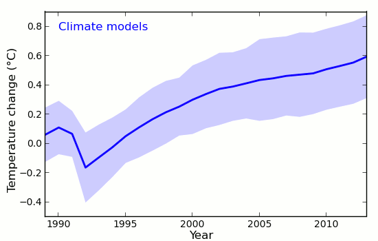
Figure 1 - The animation shows the CMIP5 model simulations compared to the HADCRUT4 surface temperature dataset. As allowances are made for better global coverage of temperature observations, El Niño/La Niña, solar radiation, and volcanic aerosols, the simulated surface temperature moves back toward the actual measured temperature over this period. Animation by Kevin C.
Still Warming After All These Years
When you consider all of Earth's reservoirs of heat; the oceans, land, ice and atmosphere together, global warming hasn't slowed down at all. In fact quite the opposite has happened, the Earth has warmed at a faster rate in the last 16 years than it did in the previous 16. Taken in isolation though, the atmosphere has bucked this trend - warming at a slower rate in the last 16 years than it did in the previous 16 years.
There was no prior scientific expectation that surface warming would progress in a linear manner, despite the ongoing build-up of heat within the Earth system, but this slower rate of surface warming comes at a time when industrial greenhouse gas emissions are larger than ever. Preying upon the seemingly common, but mistaken, public assumption of year-after-year surface warming, contrarians and some mainstream media outlets have used this opportunity to further misinform the public about global warming. One of the more popular climate myths that has emerged as a result of this counterintuitive build up of heat is that climate models have overestimated recent surface warming and therefore will overestimate future surface warming.
Climate models are computer-based mathematical calculations representing the physics of the real world, and so obviously are only rough approximations of the real Earth. It is certainly possible that they may have overestimated recent surface warming, but a closer examination of the evidence suggests any possible recent discrepancy between the models and observed surface temperatures may simply be a result of incorrect input into the models over the recent period in question. Garbage in equals garbage out (GIGO) as some might put it. Before venturing down that road, however, it's time to consider the relevant background context.
Future Weather and Climate: There Can Be Only One
Climate model projections typically involve a large number of individual model simulations which are spun-up well into the past and then run forward into the future to estimate climatic features of the Earth - such as global surface temperature trends. The timing of weather-related phenomena like El Niño and La Niña, which greatly affect surface temperatures in the short-term, cannot be accurately predicted and, because small changes in weather patterns allow the simulated weather to evolve along different pathways, there is a great deal of variation between the individual model runs. For example; a model run which simulates a predominance of La Niña over a given decade is going to exhibit cooler surface temperatures than another model run which displays El Niño dominance over the same decade. Over longer intervals, however, there may not be much difference in projected surface temperatures between the two model runs.
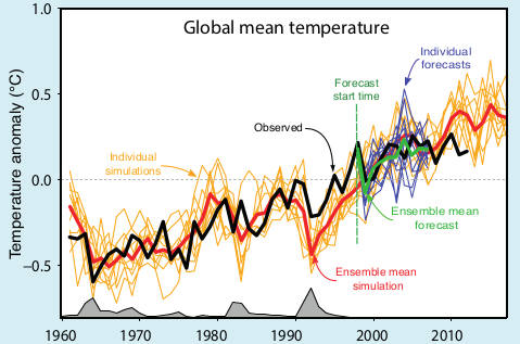
Figure 2 - A typical graphic displaying climate model simulations of global surface temperature. The spaghetti-like individual model runs are shown in orange lines. Image from the IPCC AR5 Box 11.1 Figure 1.
Multi-Model Averaging Obscures Natural Variation
Often when researchers plot the output of a batch of climate model simulations they do so by averaging all the individual runs together, known as the multi-model mean, and illustrate the uncertainty range of all the projections. The average of the model runs is shown as the thin blue line in Figure 1, and the uncertainty range of 5-95% is the blue band in the figure. The uncertainty range means that, based on all the model runs, model projections remain within the blue band 90% of the time, and 10% of the time they are either above (5%) or below (5%).
This is equivalent to some god-like experiment where we are able to run the Earth's weather forward in time over and over again, observe how global surface temperatures evolve, and then plot the output. Of course the Earth only gets one roll of the dice, so the real world is actually equivalent to only one realization of the many climate model simulations, and 90% of the time could be anywhere within the 5-95% uncertainty envelope. The multi-model mean is therefore somewhat misleading in that it obscures the inherent variability in surface temperatures in each individual model simulation. We simply do not expect temperatures at the surface in the real world to progress as smoothly as the multi-model mean would seem to imply.
Garbage In Equals Garbage Out
Due to the inability to predict the timing of natural changes within the climate system itself, such El Niño and La Niña, and factors external to the system, such as light-scattering aerosols from volcanic eruptions and industrial pollution, it becomes difficult to ascertain whether the climate model projections are diverging from reality or not. Not until the projected temperatures actually occur in the real world and persistently move outside the uncertainty range would we be aware that there was a problem.
One way to test usefulness of the climate models is to look at hindcasts - model simulations of the past where we have a reasonably good idea of what net forcing the Earth's climate was responding to. This isn't as simple as it might seem. For example; although we have a good idea of the forcing from industrial greenhouse gas emissions (which trap heat in the oceans and atmosphere), because of observational difficulties, we only have a very rough idea of the cooling effect of those tiny particles in the air called aerosols.
Not only do aerosols scatter incoming sunlight by wafting about in the atmosphere, but they also seed clouds with smaller-than-normal condensation nuclei - extending cloud lifetime. These smaller nuclei also make clouds whiter and thus more reflective to incoming sunlight. The changes in cloud characteristics imparted by aerosols (called the indirect effect) is their dominant influence and just so happens to be extraordinarily difficult to quantify. Add in the patchy and constantly changing global distribution of aerosols and it makes for a large amount of uncertainty on the forcing of surface temperatures.
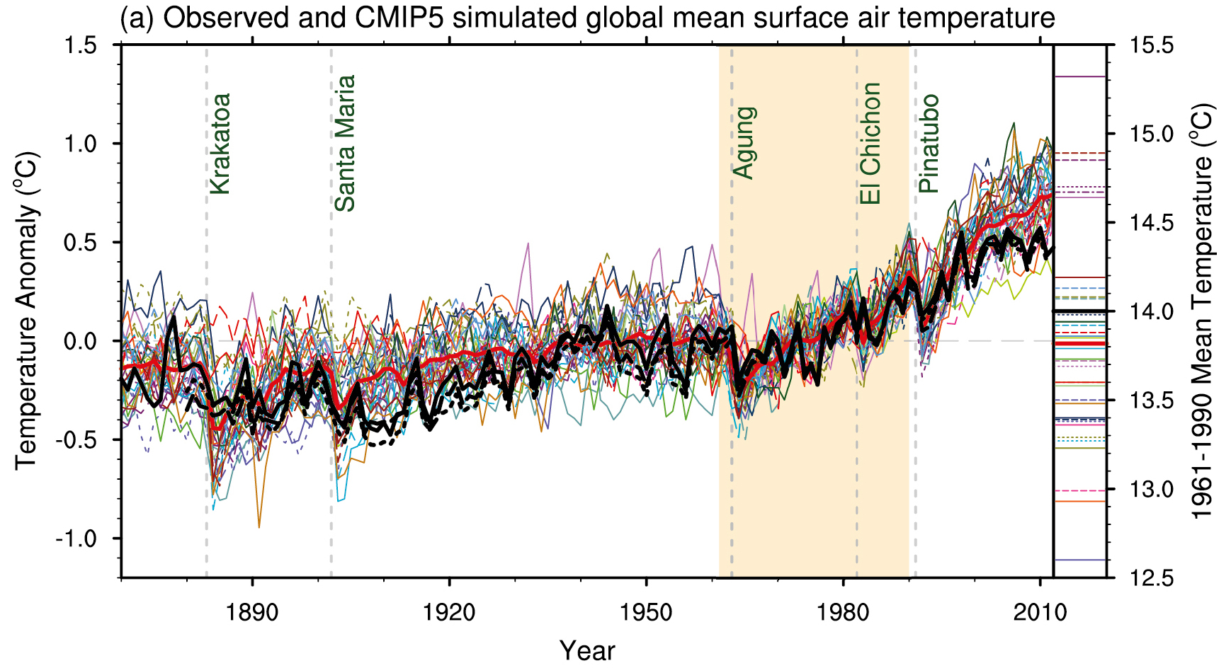
Figure 3 - CMIP5 simulations from the IPCC AR5 WG1 Figure 9.8. Black line indicates the observed global surface temperatures and the coloured lines are the climate model runs.
Schmidt (2014): Replacing CMIP5 Estimates With Better Ones
As shown in Figure 3, the collection of climate models used in the latest IPCC report (CMIP5) do a reasonable job of simulating the observed surface temperatures in the 20th century, but seem to be running too warm for the 21st century. An immediate reaction might be that the models are overestimating recent surface warming, however, given that they simulate the 20th century temperature trend with reasonable fidelity, this doesn't pass muster as a reasonable explanation. What about the long periods in the 20th century where the models do very well? And what about periods, such as the 1960's where the models run too cool? A more likely explanation is that the presumed forcings input into the model simulations, especially over the latter period could be the problem. A recently published research paper, Schmidt (2014), shows that this may indeed be the case.
When utilizing the climate models to project future surface temperature trends certain presumptions have to be made because of external influences on the climate system. Not only do industrial greenhouse gas emissions have to be estimated, but estimates are also made on the behaviour of solar radiation from the sun, and the amount and distribution of light-scattering aerosols in the atmosphere from both natural and human-made sources. In the CMIP5 simulations (shown in Figure 3) the estimated trends for the 21st century were based upon 20th century trends continuing on into 21st century (Taylor [2012], IPCC AR5), but the updated estimates and observations provided by Schmidt (2014) reveal that this did not happen. See figure 4 below.
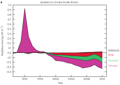
Figure 4 - updated forcing estimates of solar, volcanic, and industrial pollution for the CMIP5 climate model simulations. Image from Schmidt et al (2014).
Based on new observations, improved satellite retrievals, and reanalysis of older data, Schmidt (2014) discovered that the models overestimated the short-term cooling effect of the Mt Pinatubo eruption in 1991, and underestimated the cooling effect of increased volcanic eruptions, industrial pollution, and weaker-than-expected solar radiation in the 21st century. In comparison with the NASA surface temperature dataset, about 33% of the discrepancy in the last 16 years between the CMIP5 multi-model mean and Schmidt (2014) arises due underestimated volcanic emissions, around 15% due to weaker solar activity and El Niño/La Niña timing, and 25% due to industrial pollution.
CMIP5: The Warming That Never Was?
Rather than the models diverging from reality in recent times, as the CMIP5 models seemed to suggest, it turns out that the data fed into the simulations covering the last two decades was most likely wrong. Of course, this is not going to be the last word on the matter as the uncertainty of the size of the cooling effect of aerosols remains very large. Future observations and improved analysis could either enlarge or reduce the discrepancy further - only time will tell. As it currently stands, when corrected for the cooling and warming influences on Earth's climate, the climate models demonstrate a remarkable agreement with recent surface temperature warming trends.


Current Locations of the Net Energy Gain by the Earth over the Past 40 Years (According to the IPCC AR5) http://j.mp/EarthEnergyAllocation
I have been using this argument with opponents of ACC, and rarely get a coherent response. I also include the apparent ocean heating from Argo as another factor, and that if it was not for CO2 global temps should have fallen significantly with all these factors. so current high plateau global temps are actually strong support for ACC.
My positon is that if this is an ad hoc argument designed to shore up the fradulent alarmist cries of CAGW, then the fixes should be clunky and increasingly untenable. Much like epicycles were for the solar system.
I always acknowledge that it is possible that these are not factors, but I don't know enough about quantifying the effect, and can't read Gavin's paper (paywall).
At some point, unless these particular mitigating factors become stronger, the GHE will have to overwhelm then and global surface temps will increase and stay above current global temps. So what period of time from now would undermine current ACC theory?
tonydunc - If the models when run with accurate forcings continue to reproduce observations, and there is no time span of divergence, the 'time period' question is moot.
This post simply demonstrates that the CMIP5 model runs weren't done with the exact forcings from the last few decades, and that if those actual instances of natural variance are taken into account that the models are quite good.
"When you consider all of Earth's reservoirs of heat; the oceans, land, ice and atmosphere together, global warming hasn't slowed down at all"
Then again has it accelerated? The suggestion of this post is that warming has in fact accelerated if you include all the heat resevoirs, including ice melting and the deep ocean. I assume that means the predicted radiative imbalance has grown larger, which is what the models predict with rising GHGs.
We have a number of metrics to verify this, not the least being ocean heat content. However, there are problems with the metric of ocean heat, at least for the deep ocean in that the data are extremely sparse prior to 2005 or so when the ARGO network gained a robust density of floats.
A better metric is sea level since it includes both thermosteric and net ice melt, and it is relatively noise free. There are problems with sea level too of course, namely the satellite data only start in 1993 and the readily available tide gauge compilations readily end in 2009 so are getting kind of stale.
However, in neither of these sea level datasets do we see evidence of recent acceleration. If anything the reverse is true as evidenced by this paper at this link:
http://www.nature.com/nclimate/journal/vaop/ncurrent/full/nclimate2159.html#auth-1
The linked paper explains the lack of recent sea level rise as related to changes in the hydrologic cycle in turn related to ENSO. However, regardless, corrected sea level shows no acceleration so the claim that there has been recent acceleration of warming is dubious.
Klapper, what makes you say Sea level rise is realtivel noise free? I was under the impression that it is extremely noisy in the short term.
I remember deneirs crowing that Sea level was actually decreasing and ridiculed the notion of that being due to extreme flooding in 2012. months later sea levels shot up supporting that asessment.
Probably the best estimate of ocean warming is Balmaseda et al (2013) because, amongst other things, it combines multiple datasets and feeds these into an ocean model - thus accounting for known physics. This provides a more robust estimate for sparse or missing data.
Here's the ocean heat content trend:
What you will notice is that there an abrupt spike in heat uptake in the early 2000's followed by a slower rate up toward the present. This trend is probably one of the most obvious features of the Hiroshima Widget too.
So even though the total uptake of heat into the Earth system is greater in the last 16 years than the previous 16 years, it has not steadily accelerated. It would, therefore, be illogical to expect sea level rise to exhibit ongoing acceleration when one of the main contributors (thermal expansion) hasn't. The Cazenave et al (2014) paper seems more in line with mainstream scientific expectations, although that isn't the final word either.
Yes, tonyd, sea level can vary quite a bit and can be quite noisy. The same heat that warms and expands the ocean also lofts more water into the air and then onto land, where it can stay in some cases long enough to alter ocean levels. It may take a few years for the signal to become perfectly clear, but the latest measurements from Greenland and Antarctica show that we're in for accelerating sea level rise from here on out.
If the 2015 El Nino projections are true and we experience a temperature spike similar to the 1997-1998 El Nino, and the current solar cycle also reaches a maximum of intensity during the years 2015-2016 and if China begins to more agressively scrub its SOx emissions then we may see a significant spike in warming on a global average over the next few years.
Recent shifts in the jetstream may be harbingers of larger shifts in the global hydrological flows. If this is the case then the added tropical atmospheric moisture associated with the El Nino flow may produce a stark shift in global weather patterns.
"Some sources suggest that > 40% of Argo floats are either non- operational or produce questionable data"
Let me guess, these 'sources' don't happen to be oceanographers, but are instead non-experts ideologically resistant to the whole idea of climate-driven policy?
If readers are interested in the robustness of ocean heat measurements they should consider the IPCC AR5, Abraham et al (2013) & Von Schuckmann et al (2013). Yes the oceans are warming and the consequent thermal expansion of seawater is one of the main contributors to sea level rise.
IPCC AR5 Chapter 3 states:
"It is virtually certain that upper ocean (0 to 700 m) heat content increased during the relatively well-sampled 40-year period from 1971 to 2010"
&
"Warming of the ocean between 700 and 2000m likely contributed about 30% of the total increase in global ocean heat content (0 to 2000m) between 1957 and 2009. Although globally integrated ocean heat content in some of the 0 to 700m estimates increased more slowly from 2003 to 2010 than over the previous decade, ocean heat uptake from 700 to 2000 m likely continued unabated during this period."
As for the models, see figure 3 in the post. CMIP5 seems to do a reasonable job of simulating surface temperatures over the last hundred years. With better forcing estimates going back in time they might do an even better job. It's certainly plausible based on the work of Schmidt et al (2014).
I would also point out that Argo data is not an input into models.
@tonydunc #5:
"Klapper, what makes you say Sea level rise is realtivel noise free?"
Do a rolling R-squared using a 10 year period on the sea level data (satellite or tide guage) and compare it to the same metric on any atmospheric data set (also a 10 year period). A crude comparison but the results show sea level have much lower deviation than other climate metrics.
@jja #9:
"...and the current solar cycle also reaches a maximum of intensity during the years 2015-2016"
That is highly unlikely since the official start of solar cycle 24 is Jan 2008. A 2016 peak would put the cycle 24 peak at least 7 years after the start of the cycle, which is highly implausible.
The thermal inertia of the climate system means that the temperature takes time to respond to a change in forcing. In the case of the solar forcing, the temperature response is expected to lag the forcing by 30-50 degrees, or 11-18 months. So even if we have just passed the peak of the solar cycle, the peak effect on temperatures may not occur for another year. (And of course solar cycles are rather variable in length.)
See for example:
Knowing quantitavely what we do now about the different forcings how good are predictions or projections regarding global surface temperatures for the next 10 years?
I'm sure that volcanoes and ENSO still can't be predicted. But what about solar and aerosols. How broad should the uncertainty band around the ensemble mean be for the year 2024?
Please help me understand. Do any of the models actually fit the data or are we just saying that if we look at all the models their dispersion sort of covers a range wide enough that the real data fall within?
Can you tell me how many adjustable parameters there are in each of these models? (-snip-).
I understand that at any given time, each model is fit to the historical data and the adjustable parameters are calculated. If it fits with a good correlation, that's great, but the test of the model is whether future data fits what the model predicts. It's not good science to take the future data, refit the adjustable parameters and then report that the model fits. That usually indicates that there probably is some important physical issue that is either not in the model or not being considered correctly - maybe something like cloud formation?
If you want to put a parameter into the model that does some cooling if a volcano explodes or a La Niña happens, that's ok, but only if you do it in a way that incorporates it without using the result to readjust the fit. (-snip-).
If someone can take just one model and show how it has predicted the 10 years after the parameters were fit, I would be very appreciative.
[DB] Sloganeering, intimations of fraud and misconduct snipped. Further, the posting rights of your previous account here have been terminated since you created this one.
Please note that posting comments here at SkS is a privilege, not a right. This privilege can and will be rescinded if the posting individual continues to treat adherence to the Comments Policy as optional, rather than the mandatory condition of participating in this online forum.
Moderating this site is a tiresome chore, particularly when commentators repeatedly submit offensive or off-topic posts. We really appreciate people's cooperation in abiding by the Comments Policy, which is largely responsible for the quality of this site.
Finally, please understand that moderation policies are not open for discussion. If you find yourself incapable of abiding by these common set of rules that everyone else observes, then a change of venues is in the offing.
Please take the time to review the policy and ensure future comments are in full compliance with it. Thanks for your understanding and compliance in this matter.
The output of the climate models depend on the input. The CMIP5 climate models were fed input, a net climate forcing, that does not appear to have occurred. When fed the updated input, the multi-model mean and observed temperatures are well-matched.
None of this has anything to do with adjusting how the models themselves are run.
As for hindcasts, similar problems remain. What net forcing was the climate system itself actually responding to back then? Earlier periods are less well contrained by observations, so we can only make an educated best guess.
And one last thing, the thrust of your comment constitutes a breach of the comments policy namely; slogan-chanting and accusations of scientific malfeasance. Further breaches will likely attract moderation.
Matzdj read the post again. Models can't predict elninos/laninas, solar forcing or volcanic eruptions. No one can predict them. This post is just showing that when you take out these effects on the climate system, the models are spot on.
Martin, model are not skillful at decadal level predictions. There is a very good reason why climate is defined as 30 year means. Besides ENSO and solar variation, there are modes of internal variability on decadal scales. The models are good at predicting what 30 year trends will be however. The AR5 report indicates the ensemble range. I would say the uncertainty band is at least as large as this. Emissions and aerosols are under our control so model can only deal with scenarios for these.
Matzdj asks an interesting question:
The question doesn't really apply, because climate models are not statistial models. However from the point of view of fitting global mean temperature, I think the most meaningful answer would be 1 - because we align the baselines to compare the models.
Climate models are optimised by improving the physics. In some cases the physics cannot be modelled at a sufficiently fine scale, and in these cases parameters are used. However those parameters are not, and cannot be, optimised to reproduce global mean temperature - they are optimised to produce the right local behaviour. The global impact of those optimisations is an emergent property, and may improve or degrade the fit.
Of course we then get into the tuning myth, which was explored in another recent discussion - from memory I think we found that it arose in part from not counting the number of independant models correctly, and has changed signs between CMIP3 and 5.
@scaddenp #19:
"The models are good at predicting what 30 year trends will be however."
The current HadCRUT4 SAT trend for the last 30 years is 0.17C/decade +/- .05. The CMIP5 ensemble SAT trend for the same period (1984 to 2013 inclusive) is 0.26C/decade, which is outside the 2 sigma range of the empirical data. I checked the CMIP5 ensemble for both 80 to -90 and 90 to -90 (pole to pole) to see if the leaving the very high arctic out would improve, but it makes essentially no difference (0.26 compared to 0.25).
But that's the wrong uncertainty. The uncertainty in the trend arises from the derivation of the temperature series from linearity. The uncertainty we need for that comparison is the uncertainty due to internal variability, which will generally be larger because it also includes differences in trend. There is also doubt as to whether model spread is a good measure of this.
Matzdj, climate models are not intended for predicting the forcings (greenhouse gas emissions volcanic emissions, solar energy hitting the Earth, etc.), nor does anyone use them for that. Instead, climate models are intended for, and used for, "predicting" the climate response to one particular "scenario" of forcings. I put "predicting" in quotes, because the model run is not a genuine claim that that climate will come to pass, because there is no claim that that scenario of forcings will come to pass. Instead, the term "projecting" often is used instead of "predicting," to indicate that that climate is predicted to come to pass only if that particular scenario of forcings comes to pass. Those scenarios of forcings are the model "inputs" that other commenters have mentioned in their replies to you.
For each scenario of forcings that someone thinks might come to pass, that person can use those forcings as inputs to climate models to predict the resulting climate. To cover a range of possible scenarios, people run the climate models for each scenario to see the resulting range of possible climates. You can see that, for example, in Figure 4 in the post about Hansen's projections from 1981. You can also see it in the post about Hansen's projections from 1988. To learn about the forcings scenarios being used in the most recent IPCC reports, see the three-post series on the AR5 Representative Concentration Pathways.
To judge how well the climate models predict climate, we must input to those models the actual forcings for a given time period, so that we can then compare the models' predictions to the climate that actually happened in the real world where those particular forcings actually came to pass. That is the topic of the original post at the top of this whole comment stream.
To judge whether climate models will predict the climate in the future whose forcings we do not yet know, we must guess at what the forcing will be. We do that for a range of forcing scenarios. The bottom line is that every single remotely probable scenario of forcings yields predictions of dangerous warming.
Matzdj - Climate models predict what the climate will do over the long haul given a particular set of forcings.
Climate models do not predict economic activity (or the GHGs and industrial aerosols produced), they do not predict volcanic eruptions, they do not predict the strength of the solar cycle, and while many of them include ENSO-like variations, they do not predict _when_ those El Nino or La Nina conditions will actually occur.
Various projections (what-if scenarios) have been run for the IPCC reports with reasonable estimates of those forcings variations, but it is entirely noteworthy that the CMIP3 and CMIP5 runs did not include the _particular_ set of variations over the last few years as actually occurred - that would have required precognition. And as per the opening post, when those _actual_ variations are taken into account rather than the before-hand projections, the climate models do indeed give a good reproduction of real climate behavior.
Which means that those models continue to be reasonably accurate representations of the Earths climate, and have not been invalidated in any way whatsoever.
Matzdj, you wrote "Do any of the models actually fit the data or are we just saying that if we look at all the models their dispersion sort of covers a range wide enough that the real data fall within?"
Your question is ill-formed, because you have not specified what "actually" means. No prediction in any branch of science ever is perfect; it is valid (accurate and precise--those terms mean different things) only to some degree. Deciding whether a prediction ("projection" in our case) is sufficiently valid depends on combined probabilities and consequences of the various types of correct and incorrect actions that you could take based on your interpretation of the sufficiency of the prediction/projection.
In this case we are concerned with the projections over periods of 30 years or more (the definition of "climate"). We know that projections over shorter periods are going to be poor, especially when you get down to periods as short as ten years. But we also know that the range of those short-term projections is bound by physics ("boundary conditions"), thereby demarcating the most probable longer term (climate) range of short-term projections. Those squiggly thin orange lines in Figure 2 above are individual runs of models. The models differ from each other by design, most having been built by different people. Usually each model also is run multiple times, varying some factors as a way of sampling the range of their possible behaviors since we are confident only in a particular range of those behaviors. It's similar to running an experiment multiple times to prevent being misled by one particular random set of circumstances. The high and low extents of those squiggly orange lines represent a reasonable estimate of the bounds of the temperature.
Perhaps you are being misled by a belief that if we cannot predict short term temperature we cannot predict long term temperature. That is a common but incorrect belief. See the post "The Difference Between Weather and Climate," and Steve Easterbrook's balloon analogy on his Serendipity site.
Matzdj, understandably you might misunderstand what a "hindcast" is. It is produced in the same way as a forecast: The model is started very long ago--far earlier than the first year you are trying to hindcast. The model results gyrate wildly for a while as the simulated years tick by, then settle down. Eventually the model gets around to the first year you are trying to hindcast. The model continues through the years until getting to the year in which the model is being run. As the model continues spitting out results year by year in exactly the same process it has been following since it was started up, the "hindcasts" become "forecasts" only because the years that the models are simulating switch from being earlier than this year to being in the future from this year. For example, if climatologists start running their model on their computer in the year 1998 (I'm guessing that's where the vertical green dashed line in Figure 2 falls), then the model's outputs for each of the simulated years 1960 through 1997 are labeled "hindcasts" and the outputs for the simulated years 1998 and later are labeled "forecasts." Other than that labeling, there are no differences in how the model outputs are produced or reported. There are no adjustments to the model to tune it to actual climate.
What is done on the basis of analyses of model versus past reality is, as Kevin C explained, "improvement" of the fundamental physics of the model. I put "improvement" in quotes, because the modelers try to improve the physics but do not always succeed. They base any such adjustments on fundamental physical evidence, not by simply reducing the influence of an effect because they think it will make the projections better match observations. For example, if the modelers change the modeled reflectivity of clouds, they do so based on empirical and theoretical evidence specifically about cloud reflectivity, rather than simply making clouds more reflective because the model overall showed more heating than happened in reality. The reason that Kevin C wrote that sometimes those adjustments help the overall model output's fit and sometimes they don't, is precisely because those adjustments are not merely tunings to force the model to fit the past-observed reality.
Even if the modelers do succeed in improving the model's realism in some particular, narrow way, the effect on the model's overall, ultimate projection of temperature might be worse. For example, suppose cloud reflectivity had been modeled as too low, but that incorrect bias toward too much warming was counteracting a bias toward too much cooling in the modeling of volcanic aerosols. If the modelers genuinely improve the modeling of cloud reflectivity but do not realize the too-cool bias in the modeling of volcanic aerosols, then by reducing the warming from clouds they reduce its counterbalance of the overcooling from volcanoes, and the model's overall projection of temperature from all factors becomes worse in the too-cool direction.
Matzdj, perhaps you think that we expect the actual temperature to fall exactly on the "ensemble mean" hindcast and forecast. But we don't, because that mean has far too little variability. In fact, we expect the temperature to have wild ups and downs as you see exemplified by the orange and blue skinny lines in Figure 2, because we expect there to be El Ninos and La Ninas, variation in solar radiation, volcanic eruptions, changes in human-produced aerosols due to varying economic activity, and a slew of random and semi-random factors. It would be downright shocking if actual temperature followed the ensemble mean, because that would mean all those variations in forcings and feedbacks were far less variable than we have observed so far. So we judge the match of the real temperature to the projected temperature by whether the real temperature falls within the range of the entire set of individual model runs. Even so, we expect the real temperature to fall within that range only most of the time, not all of the time. The range you see drawn as a shaded area around the ensemble mean usually is the 90% or 95% range, meaning the set of individual model runs falls within that shaded range 90% or 95% of the time. That means, by definition, we fully expect the real temperature to fall outside that range 10% or 5% of the time. So occasional excursions of the real temperature outside that range in no way invalidate the models, when "occasional" means 10% or 5% of the time.
@Tom Dayton #25:
"In this case we are concerned with the projections over periods of 30 years or more (the definition of "climate")."
To expand on my comparison of the CMIP5 mean to empirical data, I downloaded six model runs to compare to the last 30 year global SAT warming trend. Keep in mind these models use actuals up until 2000, so the model is not guessing CO2 output or any other input for the first 1/2 of the analysis period. I used rcp45 after looking at some of the emissions projections. Rcp45 has the highest sulphur emissions which given the rapid increase in emissions from China, also seems the most realistic. In any case all rcp scenarios use the same CO2 up until 2005. If there was more than one run (true for most chosen models), I used run 0 since I'm guessing that was the baseline run. The models used were CSIRO-Mk3, GISS-E2-R, GFDL-CM3, GFDL-ESM2M, HadGEM2-ES,and MPI-ESM-LR.
The results show a fairly wide range of projected trends, from a minimum of 0.22C/decade to a maximum of 0.38C/decade, with an average of 0.28C/decade, slightly higher than the CMIP5 ensemble mean of 0.26C/decade. Even using the HadCRUT4 "Hybrid" trend for the last 30 years to compare (0.19C/decade) the average of the model runs looks to have a warming rate that is too high by 40 to 50%, depending on whether you use my selection of 6, or the CMIP5 ensemble.
However, I think the models correlate well with global SAT if you end the 30 year trend analysis period in 2000. The next step is to plot a rolling 30 year trend comparison CMIP5 ensemble vs HadCRUT4 and look for bias in the models relative to major volcanic episodes, ENSO etc.
Klapper, given recent papers on issues on HadCrut4, why choose that rather than BEST or GISS?
@scandenp #29:
Best is only land is it not? Note that my calculation on the error in the model trend above uses HadCRUT4 Hybrid with a trend of 0.19C/decade over the last 30 years, which is actually higher than GISS at .172C/decade, which is only slightly higher than HadCRUT4 at .169C/decade. I don't think it will make a lot of difference but I can plot up the rolling trend for all three (NOAA, HadCRUT4 and GISS) against the rolling CMIP5. Or maybe it's best to average the anomalies for all three Global SAT datasets.
klapper @21, 28, & 30, I have downloaded the RCP 4.5 data for all 42 ensemble members from January 1961 to December 2050 from the KNMI Climate Explorer. For the 30 year trend ending December, 2013, the ensemble shows a mean trend of 0.254 C/decade, with a Standard Deviation of 0.059 C/decade. That means any trend lying between 0.136 and 0.372 C/decade lies within the prediction interval of the ensemble. All three major temperature indices plus Cowtan and Way lie within that interval, the trends being:
HadCRUT4: 0.17 +/- 0.053 C/decade (7.1%)
NOAA: 0.162 +/- 0.052 C/decade (4.6%)
GISS: 0.172 +/- 0.056 C/decade (7.6%)
Cowtan and Way (HadCRUT4 Hybrid): 0.193 +/-0.06 C/decade (12.8%)
The numbers in brackets are the percent rank of the indices among the ensemble.
For the record, the Minimum trend in the ensemble is 0.011 C/ decade, and the Median trend is 0.249 C/decade.
Clearly neither ensemble mean prediction, nor the ensemble distribution justify claim that the models are falsified by the temperature record. That is particularly the case as there are several independent reasons to expect the ensemble to over predict the trend from 1984-2013 inclusive. First, for HadCRUT4 and NOA, neither includes the entire globe and consequently both will under predict trends due to failure to represent polar amplification.
More importantly, 1984 is still close enough to the El Chichon volcanoe of 1982 for temperatures to be negatively impacted. In real life, the impact of that volcanoe was largely nullified by the strongest El Nino on record, as measured by the SOI. More generally, that El Nino represents a peak in SOI influence on temperature, which has shown a strong negative trend since then. That has culminated, in 2011 with the strongest La Nina on record:
This strong trend in SOI conditions results in a strong negative trend in temperatures not represented by any forcing, and therefore not a feature of the ensemble mean. This couples with the lower than projected forcings to strongly bias observations relative to the ensemble.
This bias can be removed for practical purposes by comparing all thirty year trends over a period or reasonably constant increases in forcing, such as that from 1961-2050, or if you prefer largely historical values, from 1961-2013. The ensemble mean trends over those periods are, respectively, 0.222 +/- 0.076 C/decade and 0.187 +/- 0.078 C/decade. All four temperature series above lie very comfortably within the prediction interval in both cases, particularly the historical interval. For the historical period, they lie in the 41st, 36th, 42nd, and 56th percentiles respectively in order of appearance on the table above.
Sorry, minimum trend for 1984-2013 was 0.114 C/decade, not 0.011 as stated.
Klapper, you do know, don't you, that the ensemble mean is not directly a predictor of the observed climate? It is an estimate of the forced response of the climate (i.e. the behaviour of the climate in response to a change in the forcings - including any feedback mechanisms). The other component is internal climate variablity (a.k.a. the unforced response or "weather noise"). The spread of the model runs is an estimate of the variation around the forced response that we could plausibly expect to see as a result of internal climate variability. This means we should only expect the observed climate to closely resemble the ensemble mean at times when the effects of internal variability are close to zero. Where we know that sources of internal variability (e.g. ENSO) have been very active, we should not expect the observations to lie close to the ensemble mean.
This is not exactly rocket science, but it is not completely straightforward either. The reasons the models are usually presented in terms of an ensemble mean and spread, is because that is the best way of portraying what the models actually project. There is no good reason to expect the observations to lie any closer to the ensemble mean than to lie within the spread of the model runs.
@Tom Curtis #31:
I'm off to work but a few quick points:
My comment is about the "goodness" of the models over 30 years. No where did I say the empirical data "falsify" the models. You make a point that in the case of the last 30, ENSO masks the true warming signal. I agree with the tail end of the trend, but not the beginning since the empirical data show a cold period from '85 to '87, possibly the delayed effect of El Chichon.
Matzdj, see also Dikran's comment on the same point as mine about the ensemble mean.
Klapper @34, consider the comparison of the ensemble mean with the three major temperature indices below. It makes it clear that the low temperatures durring 1985 and 1986 are indeed the result of El Chichon, but the elevated temperatures in 1984 are the tail end of the record breaking El Nino as I indicated. Likewise, elevated temperatures in 1987, and 1993 to 1995 are also the consequence of strong El Ninos. These all serve to reduce the observed trend relative to the ensemble mean. Likewise, the strong La Ninas in 2008 and (particularly) 2011 also reduce the observed trend, as can be clearly seen. The effect of ENSO in reducing the observed trend is, however, clearly not limited to the "tail end" as you suggest, although the "tail end" effect is probably strongest.
You say that your "...comment is about the "goodness" of the models over 30 years".
You proceed to examining that issue in a very odd way. Climate models have thousands of dependent variables that need to be examined to determine the "'goodness' of the models". Examining just one of those variables, and that over just one restricted period tells you almost nothing about the performance of the model in predicting empirical data. Using that proceedure, we could easilly decide that one model performs poorly wheras on balance across all dependent variables it may be the best performing model. Still worse, we may decide that one model performs poorly on the specific variable we assess wheras it in fact performs well, but performs poorly over just that particular period. To avoid that possibility, the correct approach is to treat each temperature series as just another ensemble member, and determine if, statistically it is an outlier within the ensemble across all periods.
Doing just that for the data I downloaded (Jan 1961 forward) over the period of overlap with emperical measurements, I find that on thirty year trends, NOAA underperforms the ensemble mean by 15.5%, HadCRUT4 by 14.4%, and GISS by 11.2% (see data below). That is, there is no good statistical reason to think that the empirical measurements are outliers; and hence no basis to consider the models to be performing poorly. Particularly given the constraints modellers are working under. (Ideally, each model should do 200 plus runs for each scenario, forming its own ensemble; and test against the empirical data as above. That way we could rapidly sift the better from the worse performing models. Alas research budgets are not large enough, and computer time too expensive for that to be a realistic approach.)
As a side note, the approximately 15% underperformance of observations relative to models is shown by other approachs as well, indicating that it is more likely than not that the models do slightly overstate temperature increases - but talk of warming rates in models "40 to 50%" to high just shows a lack of awareness of the stochastic nature of model prediction.
@Tom Curtis #36:
I think we have different definition of "good". However, I'm sure we can agree that over the last 8 years (since 2005), the correlation between the global SAT empirical data and the model projections is getting worse. Here is a chart which tracks the rolling 30 year warming rate (plotted at the end of the period) of all major SAT compilations against the CMIP5 ensemble. To deflect some of the criticism that the SAT datasets don't include the Arctic, I have compared the warming rate of the 80 to -90 latitude CMIP5 models, eliminating the highest Arctic from the warming projection.
[PS] The image you want to post must be hosted somewhere online. You cannot embed data. See details in the HTML tips in the comments policy.
@Klapper #37:
I see my graph and last sentence did not get included. Let's try again with the graph:
Klapper @37, I concluded my comment @36 by saying "... talk of warming rates in models "40 to 50%" to high just shows a lack of awareness of the stochastic nature of model prediction."
You then prove that that is the case be quoting an eight year trend. An eight years, I might add, that goes from neutral ENSO conditions to the strongest La Nina on record as measured by the SOI.
Just so you know how pointless it is to look at eight year trends to prognosticate the future (and hence to vet climate models), the Root Mean Squared Error of eight year trends relative to 30 year trends having the same central year is 0.17 (NOAA) with an r squared of 0.015 between the two series of successive trends. That is, there is almost no correlation between the two series, and the "average" difference between the two trends is very large. The mean of the actual differences is -0.04 C/decade, indicating that eight year trends tend to underestimate thirty year trends. The standard deviation is 0.17 C/decade, giving an error margin 1.7 times larger than the estimated 30 year trend. For HadCRUT4, those figures are -0.04 mean difference, and 0.18 C/decade standard deviation. Therefore, you are quoting a figure just one standard deviation away from the current 30 year trend, and well less than two standard deviations from the predicted trend from the models as proof of a problem with the models. The phrase "straining at gnats and swallowing camels" comes to mind.
And you still want to test models against a single period rather than test their performance across an array of periods as is required to test stochastical predictions!
Klapper, just a avoid pointless controversy, do you agree with the following:
1/ ENSO is the major cause of variation from trends in the absense of volcanoes.
2/ ENSO/PDO has little/no effect on 30 trends
3/ Models cannot predict ENSO and PDO
4/ A change to positive PDO will increase SAT
And a matter of interest, what is your estimate for what an El Nino of say 1.5 will be on SAT?
scaddenp @40, the most recent ensemble mean thirty year trend (Jan 1984-Dec 2013) for CMIP5 RCP 4.5 is 0.254 C /decade. In constrast, the mean thirty year trend for the ensemble from Jan 1961 to Dec 2013 is 0.187 C per decade. To Dec 2050 it is 0.222 C/decade. The cause of the unusually high trend is the occurence of the cooling effects of El Chichon and Pinatubo in the first half of the trend period, with no equivalent volcanism in the later half. So while a thirty year period is long enough so that typically volcanic influences will not influence the trend, that is not true of all thirty year periods.
The same can also be said about ENSO.
As it happens, the slope of the SOI over the period Jan, 1984 to Dec, 2013 is 0.287 per annum, or 0.042 standard deviations per annum. That works out at 1.26 standard deviations over the full period - an appreciable, though atypical, negative influence on the trend in global temperatures.
@Tom Curtis #39:
"You then prove that that is the case be quoting an eight year trend"
I think you misunderstand. I was comparing the rolling 30 year trends over the last 8 years. Over the last 8 years the SAT and CMIP5 30 year trends have been diverging sharply. That is in contrast to the period 1965 to 2005 when the 30 year trends between SAT and the models were within much closer. The model vs. empirical warming rates were also very far apart in the 1935 to 1955 period and I've discussed that issue in the past on Skeptical Science.
@scaddenp #40:
1. No. I think the main influence on trends, at least 30 years long is the state of AMO/PDO. On shorter trends, say 10 years, then yes ENSO has the dominant leverage.
2. No. I think the the PDO or some 60 year cycle based on AMO/PDO as identified by Swanson and Tsonis has very large influence over the warming/cooling rate of longer trends, i.e. 30 years.
3. Yes/No. Enso like behaviour shows up in some of the (better?) models, but we can't predict Enso more than about 6 months in advance. Some have tried to predict ENSO based on solar cycles, like the late Theodor Landscheidt. The PDO appears to switch on a 30 year period so I'm not sure I agree with your second point
4. Can't remember positive vs negative states, but I think yes I agree.
As for the Nino3.4 at 1.5 (as predicted recently for this fall/winter), I think it might give some monthly anomalies of +0.6 in early 2015.
Klapper, then perhaps you should comment on the article "It's the PDO" and update us with research on this matter.
Klapper @43, I apologize for my insufficiently carefull reading of my post. Never-the-less, looking at the effect of adding just eight years data on thirty year trends is little better than focusing on eight year trends. You are still basing your claims on the effects of short term fluctuations, albeit indirectly by their impact on the thirty year trends.
You can see this by looking at the rolling thirty year trend for the CMIP 5 ensemble mean. It initially falls to around the '67-'97 trend as the impact of the two major volcanoes in the tail end reduces the trend. After El Chichon enters the first half of the trend period, however, the trend rises to an initial peak in the '82-'12 as both volcanoes move closer to the start of the trend period. After El Chichon falls of the start, however, the trend rises, again until Pinatubo falls of the start of the trend period, at which stage the trend rapidly declines to the 2030-2050 (terminal year) mean trend of 0.23 C/decade. The timing in the changes of slope leave no doubt that those changes are the consequences of short term events on the 30 year trends.
In contrast, the observed trend (GISS) rises faster and earlier than the modelled trend, in large part due to the effects of El Chichon being largely scrubbed by an El Nino giving greater effect to the Agung eruption (1963), not to mention the large La Ninas in '74/'75. The observed trend then levels of and declines slightly as the Pinatubo erruption nears the center point (and hence minimum effect on the trend), and as the tail of the trend period enters into the period of successively weaker El Ninos and stronger La Ninas following 2005. Again the variations are short term effects.
Because they are short term effects, we can partially project the change of trend in the future. As Pinatubo moves further towards the start of the trend period, its effect on the trend will become stronger so that the observed trend will tend to rise. This will particularly be the case if the current run of increaslingly negative SOI states ends, and we return to "normal" conditions. Unlike the modelled trend, that peaks with the 1992-2022 trend, the observed trend will remain high after that as the recent strong La Ninas move to the start of the trend period, increasing the observed trend in the same way that they now decrease the observed trend.
Basing long term projections on these year to year changes in the thirty year trend is transparently a mugs game. If you want to check observed vs modelled trends, the only sensible approach is to compare the statistics across an extended period with a steady (ie, near linear) increase in forcing at as close as possible to current rates. For easily accessible data that means RCP 4.5 from about 1960-2050.
@Tom Curtis #45:
" ..looking at the effect of adding just eight years data on thirty year trends is little better than focusing on eight year trends..."
I don't agree. There has been a rapid divergence over the last 8 years between the CMIP5 projections and empirical data 30 year linear trends. You've given some reasons, namely the timing of ENSO and volcanos, but in both you are assuming both are just noise confounding the true warming signal.
In the case of ENSO I don't agree that it is just noise. But for the sake of argument let's assume ENSO is just noise. Let us also assume the models also respond correctly to volcanos, so the error between the model and SAT trend cannot be attributed to volcanic espisodes. Again, I don't agree, I think the models overcool during volcanic episodes, but for the sake of argument...
So then let us then run a rolling 30 year trend on ENSO to find the coherence between model and empirical warming trends. Since the models don't replicate ENSO, the coherence should be good in periods when the ENSO trend is neutral and not so good when the ENSO trend is either positive or negative, right?
In some periods where the ENSO trend is basically neutral, like 1936 to 1966, and 1976 to 2006, the CMIP5 trend agrees with the SAT 30 year trend. However, in other periods where the ENSO 30 year is neutral (1916 to 1946), there is significant divergence, indicating the models are in error for some reason, either incorrect treatment of aerosols, incorrect aerosol data, or possibly incorrect treatment of GHG forcing.
Likewise, in some periods where there are strong trends in ENSO, the models have good coherence with SAT, which is puzzling, since in theory they don't "know" about ENSO. Take the 1968 to 1998 period for example, there is a strong positive trend in ENSO, which should mean the models underestimate the warming. In fact in this period the models are in good agreement with the 30year SAT trend.
Thanks to all who responded to my questions above. I have two follow-ups:
1. I believe I am hearing that climate models have no constants in the models whose values are determined by fit to the actual data? is that true? I am very surprised because I have been led to believe that in some cases, for instance cloud formation, that we do not understand the physics well enough to precisely put them into the model ? Can you give me a reference to review one of these models that have no constants that need to be multiple-variable-regression-fit to actual data before they can be used for forecast?
2. I also am hearing that when you remove the effects of El Ninos, La Ninas, volcanic eruptions, etc. that what's left fits the observed data really well. How are these effects removed? How is the effect of a strong El Nino removed differently than the effect of a weak El Nino, or the effect of a big volcanic eruption versus the effect of small one?
If we understand how to remove these from the models at the correct intensity of effect, based only on physics, when they occur, then we should be able to put them into the model as zero effect when they are not occurring and then add their effect each time one does occur with the effect that was predetermined for that intensity of event.
These are major short term forcings. Why aren't they included in the models to incorporate their effect each time they occur?
Matzdj - Your first question was answered quite succinctly by Kevin C above; there are parameterizations for physics below model resolution, which are driven only by the match to observed behavior at those small scales - local physics only. There are, however, no statistically fitted parameters for global temperature response - that is an emergent result of the large scale physics, and certainly not (as you implied in your first post on this thread) a result of tuning the global model to provide a certain answer.
As to the second question, running a GCM takes quite a bit of time and effort, note the amount of computation - they are not something you want to (or can) run every afternoon, even if you have a supercomputer cluster just hanging around. The CMIP3 and CMIP5 model runs started with a specified set of forcings, including projections through the present, and were run on those common forcings for model comparison. If the set of forcings used in those sets of model runs were constantly changing, there would never be a time when all the various modellers were working from the same set of data, no way to compare models or to look at their spread.
But as to what happens when forcings don't match the projections of a few years ago, read the opening post and look at figure one.
Matzdj - My apologies, I overlooked part of your question.
"How are these effects [ENSO, volcanic action, solar changes, etc] removed?"
The scale for the effects of these variations are derived from statistical models, namely by the use of multiple linear regression of the time signatures of those variations against the time signature of temperature. See Foster and Rahmstorf 2011 and Lean and Rind 2008 for details. And in anticipation of one of your potential questions, F&R 2011 in particular examined these variations against various lag times, which means that nonlinear responses of the climate to those forcings average out to zero in the long term - any mismatch between linear/nonlinear response cancels out.
There are other methods for these scale estimates which are in general agreement - see John Nielsen-Gammons estimates of ENSO effects, or any of the many papers on the climate effects of Pinatubo.
Klapper @46, sorry for the delayed response.
1) Here are the running thirty year trends on annual inverted SOI:
To determine the trend by start and end year, subtract 15 for the start year, and and 14 for the end year. Thus for the trend shown for 1931 in the graph, it has a start year of 1916 and an end year of 1945. You will notice that it has a 30 year trend of 0.213 per annum, a trend you mistakenly describe as "ENSO ... neutral". Rather than being ENSO neutral, it is the highest thirty year trend up to that date. It is just exceeded the following year, but not again exceeded till the trend of 1954-1983 (1969).
2) Here are the successive, inverted 360 month trends in stratospheric aerosol forcing as a proxy for the impact of volcanoes:
First, I apologize for the lack of dates. My spreadsheet did not want to put them in, and as I am only posting at the moment due to insomnia, I am disinclined to push the issue. The dates given on the graph are for the first initial month, and the last terminal month of the trends. It should be noted that actual volcanic response will be both slower, and more dispersed due to thermal inertia. The trends have been inverted so that positive trends on the graph will correlate with positive trends in temperature, all else being equal.
That brings us to the key point. You point to the strongly positive thirty year trend in ENSO from 1969-1998 as being a point where we would expect divergence between models and observed temperature trends. That period, however, coincides with a period with a significant negative trend in temperatures due to volcanism, as seen above. The actual negative trend for the Jan 1969-Dec 1998 is about half that at the trough indicated, but that strongest negative trend would have been delayed due to thermal inertia. Therefore it would have coincided very closely to the period you point to, suggesting that ENSO and volcanic influences are appreciably mutually cancelling effects in that period so that the observed temperature trend will be close to that due to the underlying forcing.
It should be noted that the volcanic influence becomes positive about terminal year 2002 and becomes strongly positive thereafter - an effect felt strongly in models, but cancelled by the strongly negative ENSO trend in observations.
3) Finally, here are the RCP4.5 vs Observed trends:
You will notice that in the year 1984 on the graph (initial year Jan 1969, terminal year Dec 1998), the observed trend is greater than the model trend. The precise values are: Modelled trend - 0.148 C/decade
Observed trend - 0.162 C/decade
This is despite the fact that on average observations run cooler than the models. In fact, the baseline trend for the period is about 0.2 C /decade for models, but 0.17 C/decade for observations, showing the modelled trend to have been reduced by approximately 25% due the the effects of volcanism (and a cooling sun), whereas the observed trend is scarcely reduced at all (due the the counteracting effect from ENSO).
You will also notice the clear pattern from the exaggerated model trend due to the effects of volcanism as discussed in my prior post.
To summarize, you presented two counter examples to my claims about the interactions of volcanism and ENSO in influencing the observed and modelled thirty year trends in Global Mean Surface Temperature. One of those counter examples is shown to be invalid because, whereas you describe it as ENSO neutral, it in fact shows a strong ENSO trend, and presumed ENSO influence on temperatures. The second counter example raises a valid point, ie, that we should expect the observed trend to be exagerated relative to modelled trend for the period 1969-1998. However, that fails as a counter example because the observed trend is exagerated relative to the modelled trend over that period, and even more so once we allow for the generally slightly (15%) lower observed relative to modelled trends. Detailed examination of the data, therefore, shows your "counter examples" to be in fact "supporting instances" - and shows the general validity of the account I have laid out here.
It should be noted that I do not presume that ENSO plus the standard forcings (including volcanic and solar) are the only influences on GMST. They are not - but they are the dominant influences. So much so that accounting for them plus thermal inertia results in a predicted temperature that correlate with observed temperatures with an r squared greater than 0.92
(Note, you in fact quoted 31 year trends rather than 30 year trends. I have therefore used the nearest relevant 30 year trends in discussing your points.)