Climate Science Glossary

Term Lookup

Enter a term in the search box to find its definition.

Settings

Use the controls in the far right panel to increase or decrease the number of terms automatically displayed (or to completely turn that feature off).

Term Lookup

Settings


All IPCC definitions taken from Climate Change 2007: The Physical Science Basis. Working Group I Contribution to the Fourth Assessment Report of the Intergovernmental Panel on Climate Change, Annex I, Glossary, pp. 941-954. Cambridge University Press.

Home Arguments Software Resources Comments The Consensus Project Translations About Support

Bluesky Facebook LinkedIn Mastodon MeWe

Twitter YouTube RSS Posts RSS Comments Email Subscribe


Climate's changed before
It's the sun
It's not bad
There is no consensus
It's cooling
Models are unreliable
Temp record is unreliable
Animals and plants can adapt
It hasn't warmed since 1998
Antarctica is gaining ice
View All Arguments...


Username
Password
New? Register here
Forgot your password?

Latest Posts

Archives

Is the CO2 effect saturated?

What the science says...

Select a level... Basic Intermediate Advanced

The notion that the CO2 effect is 'saturated' is based on a misunderstanding of how the greenhouse effect works.

Climate Myth...

CO2 effect is saturated

"Each unit of CO2 you put into the atmosphere has less and less of a warming impact. Once the atmosphere reaches a saturation point, additional input of CO2 will not really have any major impact. It's like putting insulation in your attic. They give a recommended amount and after that you can stack the insulation up to the roof and it's going to have no impact." (Marc Morano, as quoted by Steve Eliot)

At-a-Glance

This myth relies on the use (or in fact misuse) of a particular word – 'saturated'. When someone comes in from a prolonged downpour, they may well exclaim that they are saturated. They cannot imagine being any wetter. That's casual usage, though.

In science, 'saturated' is a strictly-defined term. For example, in a saturated salt solution, no more salt will dissolve, period. But what's that got to do with heat transfer in Earth's atmosphere? Let's take a look.

Heat-trapping by CO2 in the atmosphere happens because it has the ability to absorb and pass on infra-red radiation – it is a 'greenhouse gas'. Infra-red is just one part of the electromagnetic spectrum, divided by physicists into a series of bands. From the low-frequency end of the spectrum upwards, the bands are as follows: radio waves, microwaves, infrared, visible light, ultraviolet, X-rays, and gamma rays. Gamma rays thus have a very high-frequency. They are the highest-energy form of radiation.

As our understanding of the electromagnetic spectrum developed, it was realised that the radiation consists of particles called 'photons', travelling in waves. The term was coined in 1926 by the celebrated physicist Gilbert Lewis (1875-1946). A photon's energy is related to its wavelength. The shorter the wavelength, the higher the energy, so that the very high-energy gamma-rays have the shortest wavelength of the lot.

Sunshine consists mostly of ultraviolet, visible light and infra-red photons. Objects warmed by the sun then re-emit energy photons at infra-red wavelengths. Like other greenhouse gases, CO2 has the ability to absorb infra-red photons. But CO2 is unlike a mop, which has to be wrung out regularly in order for it to continue working. CO2 molecules do not get filled up with infra-red photons. Not only do they emit their own infra-red photons, but also they are constantly colliding with neighbouring molecules in the air. The constant collisions are important. Every time they happen, energy is shared out between the colliding molecules.

Through those emissions and collisions, CO2 molecules constantly warm their surroundings. This goes on all the time and at all levels in the atmosphere. You cannot say, “CO2 is saturated because the surface-emitted IR is rapidly absorbed”, because you need to take into account the whole atmosphere and its constant, ongoing energy-exchange processes. That means taking into account all absorption, all re-emission, all collisions, all heating and cooling and all eventual loss to space, at all levels.

If the amount of radiation lost to space is equal to the amount coming in from the Sun, Earth is said to be in energy balance. But if the strength of the greenhouse effect is increased, the amount of energy escaping falls behind the amount that is incoming. Earth is then said to be in an energy imbalance and the climate heats up. Double the CO2 concentration and you get a few degrees of warming: double it again and you get a few more and on and on it goes. There is no room for complacency here. By the time just one doubling has occurred, the planet would already be unrecognisable. The insulation analogy in the myth is misleading because it over-simplifies what happens in the atmosphere.

Please use this form to provide feedback about this new "At a glance" section. Read a more technical version below or dig deeper via the tabs above!


Further details

This myth relies on the use of a word – saturated. When we think of saturated in everyday use, the term 'soggy' comes to mind. This is a good example of a word that has one meaning in common parlance but another very specific one when thinking about atmospheric physics. Other such words come to mind too. Absorb and emit are two good examples relevant to this topic and we’ll discuss how they relate to atmospheric processes below.

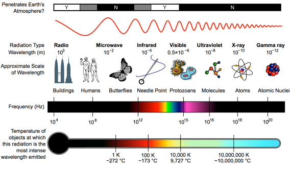
First things first. The effect of CO2 in the atmosphere is due to its influence on the transport of 'electromagnetic radiation' (EMR). EMR is energy that is moving as x-rays, ultraviolet (UV) light, visible light, infrared (IR) radiation and so on (fig. 1). Radiation is unusual in the sense that it contains energy but it is also always moving, at the speed of light, so it is also a form of transport. Radiation is also unusual in that it has properties of particles but also travels with the properties of waves, so we talk about its wavelength.

The particles making up radiation are known as photons. Each photon contains a specific amount of energy, and that is related to its wavelength. High energy photons have short wavelengths, and low energy photons have longer wavelengths. In climate, we are interested in two main radiation categories - firstly the visible light plus UV and minor IR that together make up sunshine, and secondly the IR from the earth-atmosphere system.
The Electromagnetic Spectrum

Fig. 1: diagram showing the full electromagnetic spectrum and its properties of the different bands. Image: CC BY-SA 3.0 from Wikimedia.

CO2 has the ability to absorb IR photons – it is a 'greenhouse gas'.So what does “absorb” mean, when talking about radiation? We are all familiar with using a sponge to mop up a water spill. The sponge will only absorb so much and will not absorb any more unless it's wrung out. In everyday language it may be described, without measurements, as 'saturated'. In this household example, 'absorb' basically means 'soak up' and 'saturated' simply means 'full to capacity'. Scientific terms are, in contrast, strictly defined.

Now let's look at the atmosphere. The greenhouse effect works like this: energy arrives from the sun in the form of visible light and ultraviolet radiation. A proportion reaches and warms Earth's surface. Earth then emits the energy in the form of photons of IR radiation.

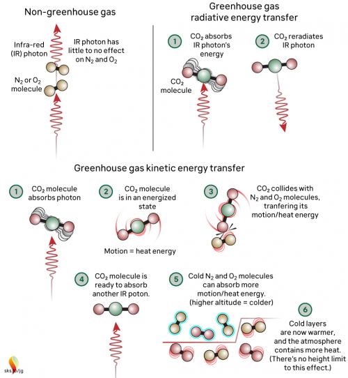
Greenhouse gases in the atmosphere, such as CO2 molecules, absorb some of this IR radiation, then re-emit it in all directions - including back to Earth's surface. The CO2 molecule does not fill up with IR photons, running out of space for any more. Instead, the CO2 molecule absorbs the energy from the IR photon and the photon ceases to be. The CO2 molecule now contains more energy, but that is transient since the molecule emits its own IR photons. Not only that: it's constantly colliding with other molecules such as N2 and O2 in the surrounding air. In those collisions, that excess energy is shared with them. This energy-sharing causes the nearby air to heat up (fig. 2).

CO2 heat transfer

Fig. 2: The greenhouse effect in action, showing the interactions between molecules. The interactions happen at all levels of the atmosphere and are constantly ongoing. Graphic: jg.

The capacity for CO2 to absorb photons is almost limitless. The CO2 molecule can also receive energy from collisions with other molecules, and it can lose energy by emitting IR radiation. When a photon is emitted, we’re not bringing a photon out of storage - we are bringing energy out of storage and turning it into a photon, travelling away at the speed of light. So CO2 is constantly absorbing IR radiation, constantly emitting IR radiation and constantly sharing energy with the surrounding air molecules. To understand the role of CO2, we need to consider all these forms of energy storage and transport.

So, where does 'saturation' get used in climate change contrarianism? The most common way they try to frame things is to claim that IR emitted from the surface, in the wavelengths where CO2 absorbs, is all absorbed fairly close to the surface. Therefore, the story continues, adding more CO2 can’t make any more difference. This is inaccurate through omission, because either innocently or deliberately, it ignores the rest of the picture, where energy is constantly being exchanged with other molecules by collisions and CO2 is constantly emitting IR radiation. This means that there is always IR radiation being emitted upwards by CO2 at all levels in the atmosphere. It might not have originated from the surface, but IR radiation is still present in the wavelengths that CO2 absorbs and emits. When emitted in the upper atmosphere, it can and will be lost to space.

When you include all the energy transfers related to the CO2 absorption of IR radiation – the transfer to other molecules, the emission, and both the upward and downward energy fluxes at all altitudes - then we find that adding CO2 to our current atmosphere acts to inhibit the transfer of radiative energy throughout that atmosphere and, ultimately, into space. This will lead to additional warming until the amount of energy being lost to space matches what is being received. This is precisely what is happening.

The myth reproduced at the top – incorrectly stating an analogy with roof insulation in that each unit has less of an effect - is misleading. Doubling CO2 from 280 ppm to 560 ppm will cause a few degrees of warming. Doubling again (560 to 1130 ppm) will cause a similar amount of additional warming, and so on. Many doublings later there may be a point where adding more CO2 has little effect, but recent work has cast serious doubt on that (He et al. 2023). But we are a long, long way from reaching that point and in any case we do not want to go anywhere near it! One doubling will be serious enough.

Finally, directly observing the specific, global radiative forcing caused by well-mixed greenhouse gases has - to date - proven elusive. This is because of irregular, uncalibrated or limited areal measurements. But very recently, results have been published regarding the deep reinterrogation of years of data (2003-2021) from the Atmospheric Infrared Sounder (AIRS) instrument on NASA's Aqua Satellite (Raghuraman et al. 2023). The work may well have finally cracked the long-standing issue of how to make finely detailed, consistent wavelength-specific measurements of outgoing long-wave radiation from Earth into space. As such, it has opened the way to direct monitoring of the radiative impact (i.e. forcing + feedback) of greenhouse gas concentration changes, thereby complimenting the Keeling Curve - the longstanding dataset of measured CO2 concentrations, down at the planet's surface.

Note: Several people in addition to John Mason were involved with updating this basic level rebuttal, namely Bob LoblawKen Rice and John Garrett (jg).

Last updated on 31 December 2023 by John Mason. View Archives

Printable Version  |  Offline PDF Version  |  Link to this page

Argument Feedback

Please use this form to let us know about suggested updates to this rebuttal.

Related Arguments

Further reading

V. Ramanthan has written a comprehensive article Trace-Gas Greenhouse Effect and Global Warming.

Further viewing

Video by Rosh Salgado on his "All about Climate" YouTube channel in which he debunks Will Happer's claim that the CO2 effect is saturated in the atmosphere:

Comments

Prev  1  2  3  4  5  6  7  8  9  10  11  12  13  14  15  16  17  18  19  20  Next

Comments 176 to 200 out of 810:

  1. For the past six days I have seen a few denialists on alt.global-warming insisting atmospheric CO2 has reached saturation point 12 years ago. At least one denialist has shown signs of hysteria over the issue, when his cherished "smoking gun" assertion gets corrected and evidence is given to him that his assertion is false. (It's like a Scientology customer learning L. Ron Hubbard's real biography; or like a Christian Scientist, who believes his legs don't really exist, trying to walk on a broken ankle.) Is there any scientist out there who believes Earth's atmosphere is CO2 saturated?
  2. 176, desertphile,
    Is there any scientist out there who believes Earth's atmosphere is CO2 saturated?
    Climate scientist? No. I'm sure you'll be able to find some physicists and such, even ones of great stature in their own fields, who will subscribe to such insanity, but not any climate scientists. Not even the likes of Roy Spencer, Richard Lindzen or Roger Pielke, Sr. [I won't link to discussions proving that Lindzen or Pielke believe in the greenhouse effect, because [snip] Suffice to say, no, not even serious deniers like Spencer, Lindzen or Pielke will destroy their own reputations that completely by ascribing to "CO2 is saturated"[snip] People who buy into lame points of view like that are either in serious denial or so thoroughly lost in the depth of the science that you can't possibly educate them.]
    Response: TC: Inflammatory snipped.
  3. Question here from a physicist educator. I have looked at these satellite comparisons between time frames. I particularly like the last in the series by Chen, et al. They look at the difference between spectra taken in two different satellites between, 1970 and 2006. But, if one were to look at outgoing IR as a function of height, does not the degree of saturation and therefore the details of the spectrum depend on the height you are measuring from? Do we care how precisely these two satellites are at the same height, here? Or perhaps all satellites are so high that the effect I am concerned about is not an issue? This is my first effort to try to understand one of these satellite papers in detail. Therefore I realize my question is probably naive to the expert.
  4. There's a very useful description of the theory, design and operational principles of the AIRS instrumentation at JPL, curiousd. How AIRS Works I'm certainly no expert but it appears the height of the instruments in this context is insignificant in the same way the distance to a star is not important when obtaining information via spectroscopy.
  5. curiousd @178, I recently created a radiative model of the atmosphere on a spreadsheet to analyze related questions. The result is that essentially all Outgoing Longwave Radiation (OLR) has its last point of emission before being radiated to space in the lower 30 km of the atmosphere, ie, from the surface, troposphere or stratosphere. Above the stratosphere, atmospheric density is so low that emissions from those altitudes are negligible. My model was too simple to include additional factors (pressure broadening of emission bands; declining CO2 content of the atmosphere above the tropopause) that would reinforce the result. Consequently any satellite, and even sufficiently high flying aircraft, will show essentially the same spectrum. You can experiment with the effect of altitude (up to 70 km) using the modtran model placed in the net by David Archer. Just compare different Iout values for different look down altitudes without changing other settings. With default settings, I obtained the following results: 70 km - 287.844 W/m^2 35 km - 287.027 W/m^2 20 km - 287.593 W/m^2 15 km - 291.863 W/m^2 10 km - 306.433 W/m^2 5 km - 348.54 W/m^2 2 km - 387.79 W/m^2
  6. Thank you, Doug Bostrom and Tom Curtis. My interest in these measurements has a different motivation than most. I am interested in presentations of the overwheming evidence for AGW and also in effective rebuttals to denialist questions. Here is a common denialist objection with which I have been blindsided.....in effect "The revolutionary treatment of CO2 and the greenhouse effect by Professor X (there exists more than one X) shows that the entire edifice of the present science is wrong. You cannot say that log 2 (Conc2/Conc1) is roughly proportional to temp increase, even for the CO2 contribution alone without feedbacks, because of the discovery of X" Rather than go to the argument that Proffessor X is not published in a standard peer reviewed jounal (will not hack it for lay audience person) or is rebutted by so and so or worse.....getting involved in real time haggling over the physics on the fly, I would prefer an experimental rebuttal. Perhaps there is such an experimental rebuttal in these papers to wit: 1. The veracity of log base two (conc2/conc1) prop to delta temp comes out of line by line computer caculations of the total CO2 absorption in the atmosphere. 2. Particularly in the article by Chen, Harries, et al the difference spectrum for CO2 between 1970 and 2006 is shown to be completely consistent with such line by line computer calculations. Therefore, All such professor X's are experimentally disproven in one stroke. Do you folks think this argument is valid?
  7. Tom Curtis 174: That is a spectacular graphic you post showing concrete environmental consequences related to climate sensitivity. But I am having trouble figuring out how to interpret this graphic, and I suspect my audience, therefore, would have more trouble. Lets see..Left hand part of the silver section..corresponds to 450 ppm with C.S. of 1.5, right? Then delta t since 1750 is about 1 degree C. The CO2 concentration is really about 380 ppm at present time with BEST showing 1.5 degrees increase at present time since 1750. Therefore BEST shows 3 degrees C.S. with 3 degrees increase since 1750 once one reaches 450 ppm. O.K. so far, since short term c.s. is now experimentally roughly 3 degrees C from many such data sets. But the viewer almost gets the quick, "sound bite take home message" that the lowest 1.5 degree C.S. case is worse than the higher C.S. cases. This I think is because the threshold temperature for the horizontal disaster line at 1000 ppm is, by this graphic, an increase of about 2.8 degrees for the 1.5 C.S. curve but the threshold temperature for the disaster line is higher for the higher C.S. curves. Which, in some sense, cannot be the case. But perhaps the key to the graph is the vertical bands of color? Then different classes of disasters are differentiated. Does bright yellow mean "hundreds of millions exposed to increased water stress"? Then by the graphic, at 380 ppm with 3 degree C.S.we should be there already.....well if you look at the American Midwest Plains these days...could be. Maybe I have that graph figured out now? Took me an hour of study, but there is a wealth of information to digest from the graph so this was study well spent,if I indeed do now understand. Then I wonder if there is away to tweak that graph toward a more rapid comprehension of the reader. If I have now interpreted the graph correctly, I will try to think of a way to do this.
  8. curiousd @182, the way to read the graph is to take a projected increase in CO2 in the lower section, and draw a line across till it intersects with a particular climate sensitivity. From that point you take a vertical line upwards to read of the expected temperature increase and environmental consequences. The graph shows an example of that procedure for the central climate sensitivity estimate at 450 ppmv (dashed lines), showing also the 95% confidence interval on climate sensitivity. The graph needs two important caveats. First, it shows only CO2 increases, but CO2 is not the only anthropogenic forcing in the atmosphere. As it happens, CO2 represents about two thirds of all anthropogenic greenhouse gas forcings, and the negative anthropogenic forcing from aerosols approximately balances the forcings from anthropogenic GHG other than CO2. Therefore, for now, the total anthropogenic forcing is approximated by that of CO2 alone. However, aerosols have a short lifetime in the atmosphere, and it is expected that as China and India develop their economy, they will follow the West in limiting the emissions of aerosol. This will increase the expected anthropogenic forcing by up to 50% above the CO2 approximation by the end of this century. On the plus side, the graph above shows the Charney (or Equilibrium) Climate Sensitivity, ie, the climate sensitivity after equilibrium is achieved with no changes to slow feedbacks like albedo from ice sheets. (Note that albedo change from changes in snow cover and sea ice are considered fast feedbacks.) The Equilibrium Climate Sensitivity takes time to be achieved. The immediate challenge is from the Transient Climate Response, which is the approximate immediate temperature impact of a slowly increasing CO2 level. It is about two thirds of the Equilibrium Climate Sensitivity (though estimates vary). This means that the estimate of current temperature increase since the pre-industrial for a 380 ppmv CO2 increase is approximately two thirds of the 1.3 C ECS, or about 0.8 C - which is a reasonably accurate prediction. That is just shy of the point where major impacts are going to be felt, according to the chart, but means there is another 0.4 to 0.5 degrees C "in the pipeline" even with no further increase in CO2. "In the pipeline", however, is an uncertain consequence. It turns out that in the short term (one to two centuries), and with no further emissions, CO2 levels fall at about the rate that the pipeline increase comes through. That means that under ideal conditions the effective increase in temperature could be limited to approximately the transient climate response. Of course, that assumes no further emissions, including from agriculture and construction, or from feedbacks such as methane release from tundra; and ignores the expected increase from reduced aerosol load. It does give us some hope of undershooting the full Equilibrium Climate Response if we genuinely initiate a zero carbon economy. Finally, the BEST temperature indice is a land only temperture, and overstates global temperature increase as a result. You should use (in order of probable accuracy) HadCRUT4, NCDC, or GISTEMP LOTI instead.
  9. Thanks again, Tom Curtis. Especially new to me is that at present, aerosols are close to offsetting the GHG effect other than CO2. Also, the good news that presently, were there to be no more CO2 emissions, CO2 should decrease enough to about cancel the rate at which the "other shoe" warming takes place. I presume - since you did not comment - that you agree with my post 181 that the results of Chen et al experimentally prove that the standard science of the CO2 greenhouse effect is correct and therefore indeed roughly every doubling of CO2 creates the same increase in temperature (about 1.2 degrees C), due to CO2 alone, with no feedbacks included?
  10. Modtran questions Thanks to info here I think Modtran on the David Archer website would be good for me to learn about. Some questions: 1. What does the water vapor parameter mean? 2. I am trying to compute the "flux weighted mean altitude of the OLR" by looking "down" from various altitudes. So with the default parameters, then at 1 Km, upward OLR flux is 406 W/m squared and so 1 Km x 406 W/m sqd is 406 Km W/m sqd And at 10 Km, upward flux is 306 w/m squared and 10 Km x 306 W/m sqd is 3060 Km W/m sqd If I keep doing this I dont think the "flux weighted mean altitude of emission to space' is well defined. It keeps getting bigger and bigger all the way up to 70 km. What am I doing wrong, here? Obviously something,or have the whole idea wrong?
  11. curiousd @185: 1) Switching between Pressure and Relative Humidity changes the way H2O concentrations are calculated with altitude. Essentially, with Pressure, H2O is a function of pressure for the standard atmosphere. As such, it will not rise nor fall if you offset the surface temperature. In contrast, with the water vapour factor set to Relative Humidity, using the surface temperature offset to increase temperature will increase the H2O concentration, while decreasing temperature will decrease it. You can explore the exact effects in greater detail by looking at the output file under atmospheric profile for H2O. 2) The method you describe will not calculate the flux weighted mean altitude of OLR. Essentially, at each altitude, z, the value recorded is the OLR from z-1 minus absorption at z, plus emissions at z. What you require is the sum of ((emissions at z - absorption of emissions from z between z and space)*z) for all z, divided by / the sum of (emissions at z - absorption of emissions from z between z and space) for all z. I strongly suspect that Modtran will not provide you with that information. If it does, it will only be by careful perusal of the output file. What may be of more interest, however, is the effective altitude of radiation, defined as the lowest altitude such that, black body radiation with an emissivity of one at the temperature of that altitude equals the total power of the OLR at TOA. The formula for the relevant temperature is, from the Stefan-Boltzman law: T= (Iout/(5.67*10^-8))^0.25
  12. Thank you. There are unexplained things in these models. Next question. If you run the "NCAR visible + IR Rad Code" for the default parameters,the first upper left hand graph shows no increase in temperature with altitude once you get to the height of the tropopause. In other words the temperature just stays constant with height after the tropopause. Is this peculiarity because there is no stratospheric ozone in the model?
  13. Never mind! Sorry. I now realize I was fooled by a cartoon drawing of the tropopause.....for an appreciable change in altitude in a realistic drawing the temp almost stays constant. Maybe that is why it is called a "pause".
  14. Question: If I run Modtran, the number given as "ground temperature" is, in the tropical atmosphere setting, the same whether I turn off all the greenhouse gases (CO2, water vapor, methane, ozone) or leave defaults. The ground temperature in the tropics is 299.7 K with or without GHG. I don't think this can be right? Help?
  15. curiousd @189, the modtran model is a Line by Line (LBL) model. That means, for a given specified set of atmospheric conditions it will calculate the IR radiation up or down at any given layer of the atmosphere from 0-70 km altitude; but it will not by itself adjust the atmospheric conditions to adjust for any change in radiative forcing. You, however, can perform the operation manually to determine the effect of a change in well mixed GHG concentration. To do so: 1) Open the model in two separate windows. 2) In the first window, set up your initial conditions. In my example this will be the default conditions of 375 ppmv CO2 and a clear sky tropical atmosphere. Note the Iout for those conditions. 3) In the second window, set "hold water vapor" to "rel hum" if you want to include the water vapour feedback, or to "pressure" if you want no feedbacks. 4) Set the change in CO2 or CH4 levels for the experiment. For my example I will double CO2 to 750 ppmv but hold CH4 constant. 5) Set the temperature offset until Iout matches that in the first window. In my example, with a water vapour feedback, that requires an offset of 1.48 C; or 0.89 C with no feedbacks. Other base settings will require different offsets. For example, for the experiment above except for mid-latitude winters, an offset of 0.77 C is required to maintain radiative equilibrium with no feedbacks; and 1 degree C with a water vapour feedback. It may seem that if you calculated the values for a number of conditions and determined area weighted values based on the area in which those conditions apply across the Earth, you could determine the the net radiative effect with an LBL model. That is not so, firstly because it only incorporates one of many feedbacks; and secondly because in the real atmosphere a change in radiative forcing will also result in changes in lateral energy transfers, so that radiative equilibrium need not be held at each location but only across the whole planet. Of course, it is easy to show with an LBL model that temperatures increases are required under all conditions with an increase in CO2 level to maintain radiative equilibrium so that the planatary Mean Surface Temperature must increase to maintain global radiative equilibrium - but that only tells you that there is an effect, not its precise magnitude. Global Circulation Models fill the gap by automatically changing atmospheric conditions at each location based on change in radiative forcing, changes in temperature, and changes in lateral energy transfer. Unfortunately, I know of no GCM with a convenient web interface like that of ModTran.
  16. Tom Curtis you have made my day!! So I shut off all the other GHG and ran Modtran with 375 PPM CO2. Wrote down outgoing flux. Kept everything the same except went to 750 ppm CO2. Adusted the temp offset to give same out going flux as before. Doubling CO2 then gives radiative energy balance for this location, if CO2 the only GHG, with a 1.1 degree C increase offset. Probably lucky but cool (pardon the expression). ( FYI Hansen says in his book that "Any physicist worth his salt can show doubling CO2 with no feedbacks gives 1.2 degree increase".)
  17. curiousd @191, the agreement is, of course, largely coincidence. One reason the model will not produce an accurate estimate of instantaneous forcing is that, unlike in the real atmosphere, increased CO2 will not result in a cooling above the tropopause. The temperature offset is relayed to all higher levels resulting in a warmer stratosphere, not a cooler stratosphere as would actually occur. Professor Brian Fiedler recommends calculating radiative forcing from 20 km look down to allow for this, which will no doubt yield better, but still imperfect results. Anyway, that is not the primary purpose of this comment. Rather, Monash University (in Melbourne, Australia) have just placed online a global energy balance model, which you may enjoy playing with. Unlike LBL models it is globally resolved, and allows for lateral energy transfers. I believe these are handled by parametrization, however, rather than being an emergent property of dynamic and radiative processes as in a GCM. As Domminget and Floter say:
    "In contrast to CGCMs the model assumes a fixed atmospheric circulation, clouds and soil moisture, which are given as boundary conditions. It thus does not simulate internal chaotic climate variability caused by weather fluctuations and also assumes that climate change, due to external forcings such as 2 9 CO2 increase, is a small perturbation, which does not change the atmospheric or ocean circulation, which is clearly a simplification."
    Clearly such a simple model cannot be used to "prove" anything; or indeed to make detailed quantitative predictions. It is potentially a useful tool for instruction (and learning), particularly as key parameters can be left out of the model to judge their influence (with suitable caveates). Full documentation of the model can be found in Domminget and Floter (2011) (PDF).
  18. Thank you again. The application of Modtran by Professor Fiedler is most illuminating. I tried the MONASH program and have given feedback to their group. Another program on David Archer's website is the NCAR radiation code. The out put table has symbols 1ev p z T q What do these mean? I am certain 1 eV cannot mean one electron volt?
  19. curiousd @193, I am not familiar with that model, so I can't be much help. However: lev = Level, numbered from the top of the atmosphere (32 km) p = atmospheric pressure at that level z = altitude in kilometers T = temperature Unfortunately I cannot help you with q.
  20. curiousd, Tom: q is almost certainly specific humidity (mass of water vapour per unit mass of moist air). Humidity units can be quite confusing - the only one that makes sense to everyone is relative humidity, and it's the one that is most useless for serious work. Other common ones: e - vapour pressure (partial pressure of water vapour) r - mixing ratio (mass of water vapour per unit mass of dry air) Td - dew point temperature (temperature at which air would reach saturation if cooled) Conversion between various forms is a common torture test subject in undergraduate meteorology courses.
  21. Hi, Thanks to the help here, and hours of struggling, I can now demonstrate some cool things with Modtran, which if used with care, is a great teaching tool. Potentially that NCAR program on the same website would also be useful. Maybe there is some kind of workshop people hold for users? In my own research field they hold such workshops at synchrotrons to help people hone their software analysis skills. If there were at least a handbook on NCAR with worked examples? Sigh! Just one example of where I go awry here, follows: 1. I find the temperature corresponding to no GHG for the default incoming solar flux. That should be T earth, which averaged over the globe would be about 255 K. 2. I go back to default and put in CO2 375 ppm. 3. The output gives you temperatures associated with various altitudes. 4. If the T earth for the setting you use were 255 K for no GHG - then go back to 3 above and write down the altitude for 255 K 5. Now try 750 ppm. The surface temperature goes up but the altitude for 255 K should go up too. It does this, but.... 6. Check against equation: change in this altitude times lapse rate = change in temperature. 6. I get a much bigger change in temperature using the altitude change method than the actual computed change in temperature. I have a feeling I am careening around in a complex vehicle randomly trying to make sense out of tweaking the controls. I probably need to go someplace to learn this one on one?
  22. Never mind, The Archer course web site has many bugs but I am able to at least learn what the parameters do by ignoring the bugs and proceeding as best I can.
  23. Now a specific question: In NACAR from Archer web site I keep everything default except I increase the high cloud fraction from zero. The temperature goes down, not up. As an amateur here I have absorbed the "high clouds tend to add to the Greenhouse Effect, low clouds tend to reflect" (over?)generalization. So why does adding high clouds cool in this NACAR program at default settings? I do not think there is a way to ask a question on line with that course.
  24. Never mind. I think I have figured out that NACAR thing pretty much now on my own now, just by persistent putzing around, day after day.
  25. Stealth, see also "A Saturated Gassy Argument" part 1 and part 2.  For more technical depth, check out Science of Doom; there are several places where saturation is discussed, but you might start with Part Five.

Prev  1  2  3  4  5  6  7  8  9  10  11  12  13  14  15  16  17  18  19  20  Next

Post a Comment

Political, off-topic or ad hominem comments will be deleted. Comments Policy...

You need to be logged in to post a comment. Login via the left margin or if you're new, register here.

Link to this page


The Consensus Project Website

THE ESCALATOR

(free to republish)


© Copyright 2024 John Cook
Home | Translations | About Us | Privacy | Contact Us