


 Arguments


Is the CO2 effect saturated?
What the science says...
| Select a level... |
 Basic
Basic
|
 Intermediate
|
 Advanced
| ||||
|
The notion that the CO2 effect is 'saturated' is based on a misunderstanding of how the greenhouse effect works. |
|||||||
Climate Myth...
CO2 effect is saturated
"Each unit of CO2 you put into the atmosphere has less and less of a warming impact. Once the atmosphere reaches a saturation point, additional input of CO2 will not really have any major impact. It's like putting insulation in your attic. They give a recommended amount and after that you can stack the insulation up to the roof and it's going to have no impact." (Marc Morano, as quoted by Steve Eliot)
At-a-Glance
This myth relies on the use (or in fact misuse) of a particular word – 'saturated'. When someone comes in from a prolonged downpour, they may well exclaim that they are saturated. They cannot imagine being any wetter. That's casual usage, though.
In science, 'saturated' is a strictly-defined term. For example, in a saturated salt solution, no more salt will dissolve, period. But what's that got to do with heat transfer in Earth's atmosphere? Let's take a look.
Heat-trapping by CO2 in the atmosphere happens because it has the ability to absorb and pass on infra-red radiation – it is a 'greenhouse gas'. Infra-red is just one part of the electromagnetic spectrum, divided by physicists into a series of bands. From the low-frequency end of the spectrum upwards, the bands are as follows: radio waves, microwaves, infrared, visible light, ultraviolet, X-rays, and gamma rays. Gamma rays thus have a very high-frequency. They are the highest-energy form of radiation.
As our understanding of the electromagnetic spectrum developed, it was realised that the radiation consists of particles called 'photons', travelling in waves. The term was coined in 1926 by the celebrated physicist Gilbert Lewis (1875-1946). A photon's energy is related to its wavelength. The shorter the wavelength, the higher the energy, so that the very high-energy gamma-rays have the shortest wavelength of the lot.
Sunshine consists mostly of ultraviolet, visible light and infra-red photons. Objects warmed by the sun then re-emit energy photons at infra-red wavelengths. Like other greenhouse gases, CO2 has the ability to absorb infra-red photons. But CO2 is unlike a mop, which has to be wrung out regularly in order for it to continue working. CO2 molecules do not get filled up with infra-red photons. Not only do they emit their own infra-red photons, but also they are constantly colliding with neighbouring molecules in the air. The constant collisions are important. Every time they happen, energy is shared out between the colliding molecules.
Through those emissions and collisions, CO2 molecules constantly warm their surroundings. This goes on all the time and at all levels in the atmosphere. You cannot say, “CO2 is saturated because the surface-emitted IR is rapidly absorbed”, because you need to take into account the whole atmosphere and its constant, ongoing energy-exchange processes. That means taking into account all absorption, all re-emission, all collisions, all heating and cooling and all eventual loss to space, at all levels.
If the amount of radiation lost to space is equal to the amount coming in from the Sun, Earth is said to be in energy balance. But if the strength of the greenhouse effect is increased, the amount of energy escaping falls behind the amount that is incoming. Earth is then said to be in an energy imbalance and the climate heats up. Double the CO2 concentration and you get a few degrees of warming: double it again and you get a few more and on and on it goes. There is no room for complacency here. By the time just one doubling has occurred, the planet would already be unrecognisable. The insulation analogy in the myth is misleading because it over-simplifies what happens in the atmosphere.
Please use this form to provide feedback about this new "At a glance" section. Read a more technical version below or dig deeper via the tabs above!
Further details
This myth relies on the use of a word – saturated. When we think of saturated in everyday use, the term 'soggy' comes to mind. This is a good example of a word that has one meaning in common parlance but another very specific one when thinking about atmospheric physics. Other such words come to mind too. Absorb and emit are two good examples relevant to this topic and we’ll discuss how they relate to atmospheric processes below.
First things first. The effect of CO2 in the atmosphere is due to its influence on the transport of 'electromagnetic radiation' (EMR). EMR is energy that is moving as x-rays, ultraviolet (UV) light, visible light, infrared (IR) radiation and so on (fig. 1). Radiation is unusual in the sense that it contains energy but it is also always moving, at the speed of light, so it is also a form of transport. Radiation is also unusual in that it has properties of particles but also travels with the properties of waves, so we talk about its wavelength.
The particles making up radiation are known as photons. Each photon contains a specific amount of energy, and that is related to its wavelength. High energy photons have short wavelengths, and low energy photons have longer wavelengths. In climate, we are interested in two main radiation categories - firstly the visible light plus UV and minor IR that together make up sunshine, and secondly the IR from the earth-atmosphere system.
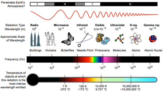
Fig. 1: diagram showing the full electromagnetic spectrum and its properties of the different bands. Image: CC BY-SA 3.0 from Wikimedia.
CO2 has the ability to absorb IR photons – it is a 'greenhouse gas'.So what does “absorb” mean, when talking about radiation? We are all familiar with using a sponge to mop up a water spill. The sponge will only absorb so much and will not absorb any more unless it's wrung out. In everyday language it may be described, without measurements, as 'saturated'. In this household example, 'absorb' basically means 'soak up' and 'saturated' simply means 'full to capacity'. Scientific terms are, in contrast, strictly defined.
Now let's look at the atmosphere. The greenhouse effect works like this: energy arrives from the sun in the form of visible light and ultraviolet radiation. A proportion reaches and warms Earth's surface. Earth then emits the energy in the form of photons of IR radiation.
Greenhouse gases in the atmosphere, such as CO2 molecules, absorb some of this IR radiation, then re-emit it in all directions - including back to Earth's surface. The CO2 molecule does not fill up with IR photons, running out of space for any more. Instead, the CO2 molecule absorbs the energy from the IR photon and the photon ceases to be. The CO2 molecule now contains more energy, but that is transient since the molecule emits its own IR photons. Not only that: it's constantly colliding with other molecules such as N2 and O2 in the surrounding air. In those collisions, that excess energy is shared with them. This energy-sharing causes the nearby air to heat up (fig. 2).
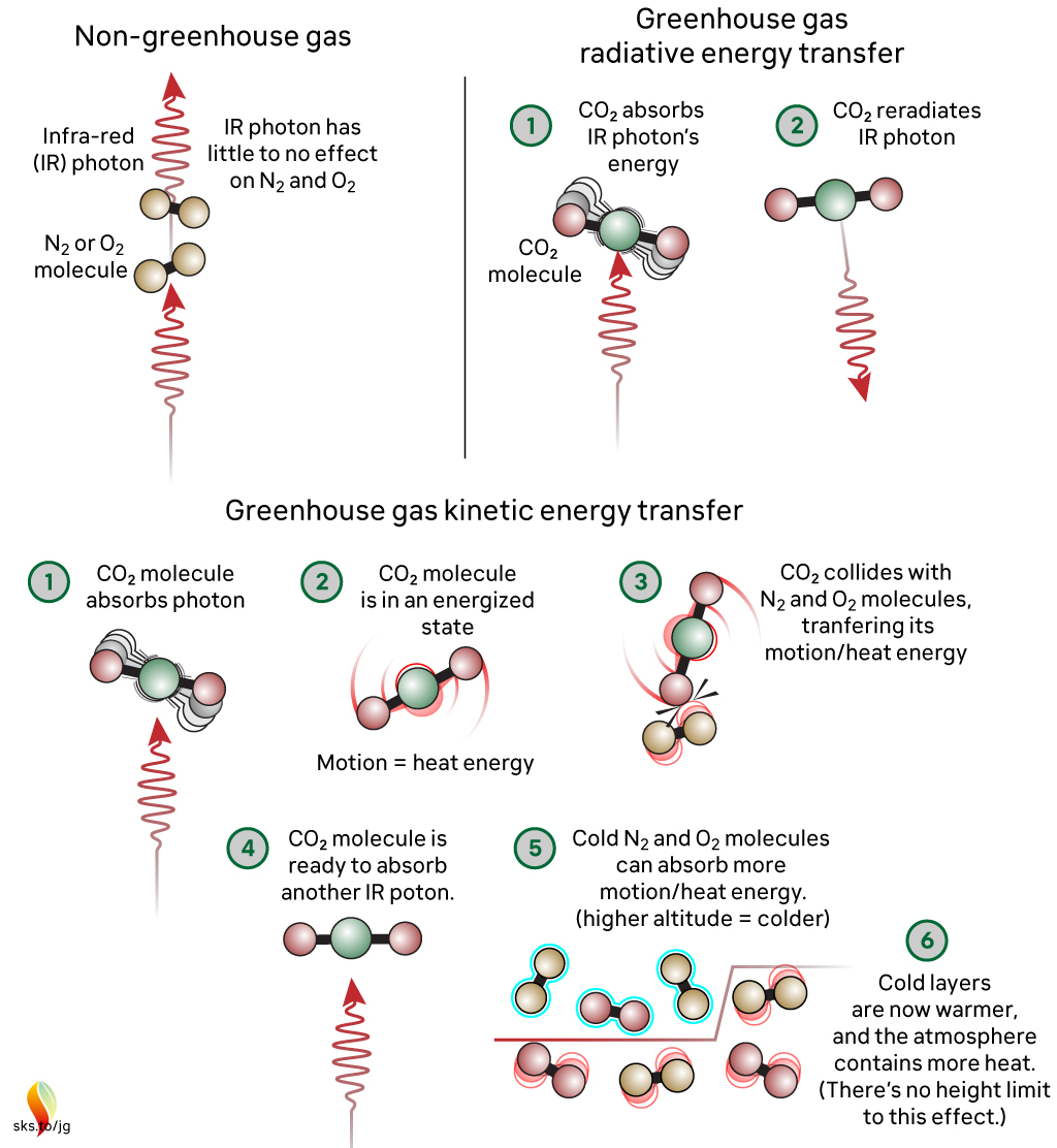
Fig. 2: The greenhouse effect in action, showing the interactions between molecules. The interactions happen at all levels of the atmosphere and are constantly ongoing. Graphic: jg.
The capacity for CO2 to absorb photons is almost limitless. The CO2 molecule can also receive energy from collisions with other molecules, and it can lose energy by emitting IR radiation. When a photon is emitted, we’re not bringing a photon out of storage - we are bringing energy out of storage and turning it into a photon, travelling away at the speed of light. So CO2 is constantly absorbing IR radiation, constantly emitting IR radiation and constantly sharing energy with the surrounding air molecules. To understand the role of CO2, we need to consider all these forms of energy storage and transport.
So, where does 'saturation' get used in climate change contrarianism? The most common way they try to frame things is to claim that IR emitted from the surface, in the wavelengths where CO2 absorbs, is all absorbed fairly close to the surface. Therefore, the story continues, adding more CO2 can’t make any more difference. This is inaccurate through omission, because either innocently or deliberately, it ignores the rest of the picture, where energy is constantly being exchanged with other molecules by collisions and CO2 is constantly emitting IR radiation. This means that there is always IR radiation being emitted upwards by CO2 at all levels in the atmosphere. It might not have originated from the surface, but IR radiation is still present in the wavelengths that CO2 absorbs and emits. When emitted in the upper atmosphere, it can and will be lost to space.
When you include all the energy transfers related to the CO2 absorption of IR radiation – the transfer to other molecules, the emission, and both the upward and downward energy fluxes at all altitudes - then we find that adding CO2 to our current atmosphere acts to inhibit the transfer of radiative energy throughout that atmosphere and, ultimately, into space. This will lead to additional warming until the amount of energy being lost to space matches what is being received. This is precisely what is happening.
The myth reproduced at the top – incorrectly stating an analogy with roof insulation in that each unit has less of an effect - is misleading. Doubling CO2 from 280 ppm to 560 ppm will cause a few degrees of warming. Doubling again (560 to 1130 ppm) will cause a similar amount of additional warming, and so on. Many doublings later there may be a point where adding more CO2 has little effect, but recent work has cast serious doubt on that (He et al. 2023). But we are a long, long way from reaching that point and in any case we do not want to go anywhere near it! One doubling will be serious enough.
Finally, directly observing the specific, global radiative forcing caused by well-mixed greenhouse gases has - to date - proven elusive. This is because of irregular, uncalibrated or limited areal measurements. But very recently, results have been published regarding the deep reinterrogation of years of data (2003-2021) from the Atmospheric Infrared Sounder (AIRS) instrument on NASA's Aqua Satellite (Raghuraman et al. 2023). The work may well have finally cracked the long-standing issue of how to make finely detailed, consistent wavelength-specific measurements of outgoing long-wave radiation from Earth into space. As such, it has opened the way to direct monitoring of the radiative impact (i.e. forcing + feedback) of greenhouse gas concentration changes, thereby complimenting the Keeling Curve - the longstanding dataset of measured CO2 concentrations, down at the planet's surface.
Note: Several people in addition to John Mason were involved with updating this basic level rebuttal, namely Bob Loblaw, Ken Rice and John Garrett (jg).
Last updated on 31 December 2023 by John Mason. View Archives


torturetest subject in undergraduate meteorology courses.Stealth, see also "A Saturated Gassy Argument" part 1 and part 2. For more technical depth, check out Science of Doom; there are several places where saturation is discussed, but you might start with Part Five.