


 Arguments


How sensitive is our climate?
What the science says...
| Select a level... |
 Basic
Basic
|
 Intermediate
|
 Advanced
| ||||
|
Net positive feedback is confirmed by many different lines of evidence. |
|||||||
Climate sensitivity is low
"His [Dr Spencer's] latest research demonstrates that – in the short term, at any rate – the temperature feedbacks that the IPCC imagines will greatly amplify any initial warming caused by CO2 are net-negative, attenuating the warming they are supposed to enhance. His best estimate is that the warming in response to a doubling of CO2 concentration, which may happen this century unless the usual suspects get away with shutting down the economies of the West, will be a harmless 1 Fahrenheit degree, not the 6 F predicted by the IPCC." (Christopher Monckton)
At-a-glance
Climate sensitivity is of the utmost importance. Why? Because it is the factor that determines how much the planet will warm up due to our greenhouse gas emissions. The first calculation of climate sensitivity was done by Swedish scientist Svante Arrhenius in 1896. He worked out that a doubling of the concentration of CO2 in air would cause a warming of 4-6oC. However, CO2 emissions at the time were miniscule compared to today's. Arrhenius could not have foreseen the 44,250,000,000 tons we emitted in 2019 alone, through energy/industry plus land use change, according to the IPCC Sixth Assessment Report (AR6) of 2022.
Our CO2 emissions build up in our atmosphere trapping more heat, but the effect is not instant. Temperatures take some time to fully respond. All natural systems always head towards physical equilibrium but that takes time. The absolute climate sensitivity value is therefore termed 'equilibrium climate sensitivity' to emphasise this.
Climate sensitivity has always been expressed as a range. The latest estimate, according to AR6, has a 'very likely' range of 2-5oC. Narrowing it down even further is difficult for a number of reasons. Let's look at some of them.
To understand the future, we need to look at what has already happened on Earth. For that, we have the observational data going back to just before Arrhenius' time and we also have the geological record, something we understand in ever more detail.
For the future, we also need to take feedbacks into account. Feedbacks are the responses of other parts of the climate system to rising temperatures. For example, as the world warms up. more water vapour enters the atmosphere due to enhanced evaporation. Since water vapour is a potent greenhouse gas, that pushes the system further in the warming direction. We know that happens, not only from basic physics but because we can see it happening. Some other feedbacks happen at a slower pace, such as CO2 and methane release as permafrost melts. We know that's happening, but we've yet to get a full handle on it.
Other factors serve to speed up or slow down the rate of warming from year to year. The El Nino-La Nina Southern Oscillation, an irregular cycle that raises or lowers global temperatures, is one well-known example. Significant volcanic activity occurs on an irregular basis but can sometimes have major impacts. A very large explosive eruption can load the atmosphere with aerosols such as tiny droplets of sulphuric acid and these have a cooling effect, albeit only for a few years.
These examples alone show why climate change is always discussed in multi-decadal terms. When you stand back from all that noise and look at the bigger picture, the trend-line is relentlessly heading upwards. Since 1880, global temperatures have already gone up by more than 1oC - almost 2oF, thus making a mockery of the 2010 Monckton quote in the orange box above.
That amount of temperature rise in just over a century suggests that the climate is highly sensitive to human CO2 emissions. So far, we have increased the atmospheric concentration of CO2 by 50%, from 280 to 420 ppm, since 1880. Furthermore, since 1981, temperature has risen by around 0.18oC per decade. So we're bearing down on the IPCC 'very likely' range of 2-5oC with a vengeance.
Please use this form to provide feedback about this new "At a glance" section. Read a more technical version below or dig deeper via the tabs above!
Further details
Climate sensitivity is the estimate of how much the earth's climate will warm in response to the increased greenhouse effect if we manage, against all the good advice, to double the amount of carbon dioxide in the atmosphere. This includes feedbacks that can either amplify or dampen the warming. If climate sensitivity is low, as some climate 'skeptics' claim (without evidence), then the planet will warm slowly and we will have more time to react and adapt. If sensitivity is high, then we could be in for a very bad time indeed. Feeling lucky? Let's explore.
Sensitivity is expressed as the range of temperature increases that we can expect to find ourselves within, once the system has come to equilibrium with that CO2 doubling: it is therefore often referred to as Equilibrium Climate Sensitivity, hereafter referred to as ECS.
There are two ways of working out the value of climate sensitivity, used in combination. One involves modelling, the other calculates the figure directly from physical evidence, by looking at climate changes in the distant past, as recorded for example in ice-cores, in marine sediments and numerous other data-sources.
The first modern estimates of climate sensitivity came from climate models. In the 1979 Charney report, available here, two models from Suki Manabe and Jim Hansen estimated a sensitivity range between 1.5 to 4.5°C. Not bad, as we will see. Since then further attempts at modelling this value have arrived at broadly similar figures, although the maximum values in some cases have been high outliers compared to modern estimates. For example Knutti et al. 2006 entered different sensitivities into their models and then compared the models with observed seasonal responses to get a climate sensitivity range of 1.5 to 6.5°C - with 3 to 3.5°C most likely.
Studies that calculate climate sensitivity directly from empirical observations, independent of models, began a little more recently. Lorius et al. 1990 examined Vostok ice core data and calculated a range of 3 to 4°C. Hansen et al. 1993 looked at the last 20,000 years when the last ice age ended and empirically calculated a climate sensitivity of 3 ± 1°C. Other studies have resulted in similar values although given the amount of recent warming, some of their lower bounds are probably too low. More recent studies have generated values that are more broadly consistent with modelling and indicative of a high level of understanding of the processes involved.
More recently, and based on multiple lines of evidence, according to the IPCC Sixth Assessment Report (2021), the "best estimate of ECS is 3°C, the likely range is 2.5°C to 4°C, and the very likely range is 2°C to 5°C. It is virtually certain that ECS is larger than 1.5°C". This is unsurprising since just a 50% rise in CO2 concentrations since 1880, mostly in the past few decades, has already produced over 1°C of warming. Substantial advances have been made since the Fifth Assessment Report in quantifying ECS, "based on feedback process understanding, the instrumental record, paleoclimates and emergent constraints". Although all the lines of evidence rule out ECS values below 1.5°C, it is not yet possible to rule out ECS values above 5°C. Therefore, in the strictly-defined IPCC terminology, the 5°C upper end of the very likely range is assessed to have medium confidence and the other bounds have high confidence.
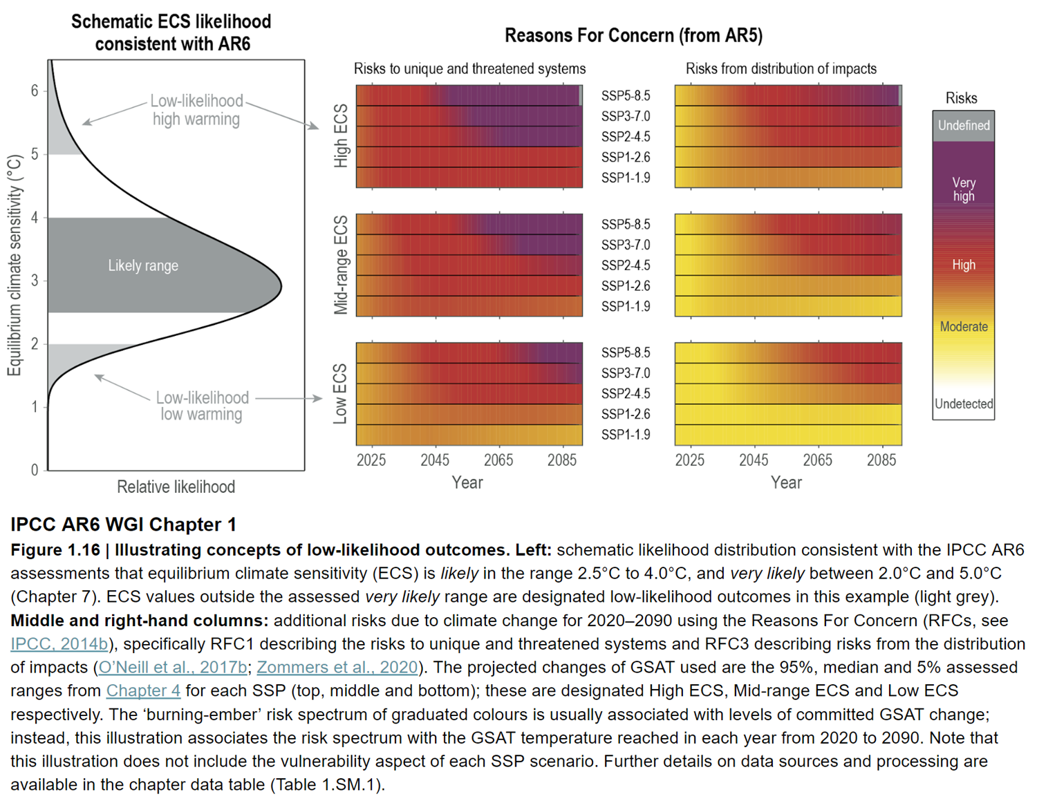
Fig. 1: Left: schematic likelihood distribution consistent with the IPCC AR6 assessments that equilibrium climate sensitivity (ECS) is likely in the range 2.5°C to 4.0°C, and very likely between 2.0°C and 5.0°C. ECS values outside the assessed very likely range are designated low-likelihood outcomes in this example (light grey). Middle and right-hand columns: additional risks due to climate change for 2020 to 2090. Source: IPCC AR6 WGI Chapter 6 Figure 1-16.
It’s all a matter of degree
All the models and evidence confirm a minimum warming close to 2°C for a doubling of atmospheric CO2 with a most likely value of 3°C and the potential to warm 4°C or even more. These are not small rises: they would signal many damaging and highly disruptive changes to the environment (fig. 1). In this light, the arguments against reducing greenhouse gas emissions because of "low" climate sensitivity are a form of gambling. A minority claim the climate is less sensitive than we think, the implication being that as a consequence, we don’t need to do anything much about it. Others suggest that because we can't tell for sure, we should wait and see. Both such stances are nothing short of stupid. Inaction or complacency in the face of the evidence outlined above severely heightens risk. It is gambling with the entire future ecology of the planet and the welfare of everyone on it, on the rapidly diminishing off-chance of being right.
Last updated on 12 November 2023 by John Mason. View Archives
 @164 and 165, I don't know, but that seems the most natural reading to me. You should always take average to mean "mean", not "weighted mean" (or median or mode) unless there are clear contextual reasons to think otherwise. There are no such contextual reasons here; and furthermore, your discreprancy gives weight to that interpretation. Which is more likely, that a program developed by the air force for research and which has been used in various incarnations since 1988 with good correspondence to observational results has an error that produces up to 20% errors in its output? Or that you are simply mistaken in your interpretation of average?
Regardless, if you disagree with me, you do the LBL integration. I am not the one chasing windmills here.
@169, no, you just add up the individual lines. Any divisions (if necessary, see 163) shoud be done for each line only.
@164 and 165, I don't know, but that seems the most natural reading to me. You should always take average to mean "mean", not "weighted mean" (or median or mode) unless there are clear contextual reasons to think otherwise. There are no such contextual reasons here; and furthermore, your discreprancy gives weight to that interpretation. Which is more likely, that a program developed by the air force for research and which has been used in various incarnations since 1988 with good correspondence to observational results has an error that produces up to 20% errors in its output? Or that you are simply mistaken in your interpretation of average?
Regardless, if you disagree with me, you do the LBL integration. I am not the one chasing windmills here.
@169, no, you just add up the individual lines. Any divisions (if necessary, see 163) shoud be done for each line only.


Climate Myth...