


 Arguments


How sensitive is our climate?
What the science says...
| Select a level... |
 Basic
Basic
|
 Intermediate
|
 Advanced
| ||||
|
Net positive feedback is confirmed by many different lines of evidence. |
|||||||
Climate Myth...
Climate sensitivity is low
"His [Dr Spencer's] latest research demonstrates that – in the short term, at any rate – the temperature feedbacks that the IPCC imagines will greatly amplify any initial warming caused by CO2 are net-negative, attenuating the warming they are supposed to enhance. His best estimate is that the warming in response to a doubling of CO2 concentration, which may happen this century unless the usual suspects get away with shutting down the economies of the West, will be a harmless 1 Fahrenheit degree, not the 6 F predicted by the IPCC." (Christopher Monckton)
At-a-glance
Climate sensitivity is of the utmost importance. Why? Because it is the factor that determines how much the planet will warm up due to our greenhouse gas emissions. The first calculation of climate sensitivity was done by Swedish scientist Svante Arrhenius in 1896. He worked out that a doubling of the concentration of CO2 in air would cause a warming of 4-6oC. However, CO2 emissions at the time were miniscule compared to today's. Arrhenius could not have foreseen the 44,250,000,000 tons we emitted in 2019 alone, through energy/industry plus land use change, according to the IPCC Sixth Assessment Report (AR6) of 2022.
Our CO2 emissions build up in our atmosphere trapping more heat, but the effect is not instant. Temperatures take some time to fully respond. All natural systems always head towards physical equilibrium but that takes time. The absolute climate sensitivity value is therefore termed 'equilibrium climate sensitivity' to emphasise this.
Climate sensitivity has always been expressed as a range. The latest estimate, according to AR6, has a 'very likely' range of 2-5oC. Narrowing it down even further is difficult for a number of reasons. Let's look at some of them.
To understand the future, we need to look at what has already happened on Earth. For that, we have the observational data going back to just before Arrhenius' time and we also have the geological record, something we understand in ever more detail.
For the future, we also need to take feedbacks into account. Feedbacks are the responses of other parts of the climate system to rising temperatures. For example, as the world warms up. more water vapour enters the atmosphere due to enhanced evaporation. Since water vapour is a potent greenhouse gas, that pushes the system further in the warming direction. We know that happens, not only from basic physics but because we can see it happening. Some other feedbacks happen at a slower pace, such as CO2 and methane release as permafrost melts. We know that's happening, but we've yet to get a full handle on it.
Other factors serve to speed up or slow down the rate of warming from year to year. The El Nino-La Nina Southern Oscillation, an irregular cycle that raises or lowers global temperatures, is one well-known example. Significant volcanic activity occurs on an irregular basis but can sometimes have major impacts. A very large explosive eruption can load the atmosphere with aerosols such as tiny droplets of sulphuric acid and these have a cooling effect, albeit only for a few years.
These examples alone show why climate change is always discussed in multi-decadal terms. When you stand back from all that noise and look at the bigger picture, the trend-line is relentlessly heading upwards. Since 1880, global temperatures have already gone up by more than 1oC - almost 2oF, thus making a mockery of the 2010 Monckton quote in the orange box above.
That amount of temperature rise in just over a century suggests that the climate is highly sensitive to human CO2 emissions. So far, we have increased the atmospheric concentration of CO2 by 50%, from 280 to 420 ppm, since 1880. Furthermore, since 1981, temperature has risen by around 0.18oC per decade. So we're bearing down on the IPCC 'very likely' range of 2-5oC with a vengeance.
Please use this form to provide feedback about this new "At a glance" section. Read a more technical version below or dig deeper via the tabs above!
Further details
Climate sensitivity is the estimate of how much the earth's climate will warm in response to the increased greenhouse effect if we manage, against all the good advice, to double the amount of carbon dioxide in the atmosphere. This includes feedbacks that can either amplify or dampen the warming. If climate sensitivity is low, as some climate 'skeptics' claim (without evidence), then the planet will warm slowly and we will have more time to react and adapt. If sensitivity is high, then we could be in for a very bad time indeed. Feeling lucky? Let's explore.
Sensitivity is expressed as the range of temperature increases that we can expect to find ourselves within, once the system has come to equilibrium with that CO2 doubling: it is therefore often referred to as Equilibrium Climate Sensitivity, hereafter referred to as ECS.
There are two ways of working out the value of climate sensitivity, used in combination. One involves modelling, the other calculates the figure directly from physical evidence, by looking at climate changes in the distant past, as recorded for example in ice-cores, in marine sediments and numerous other data-sources.
The first modern estimates of climate sensitivity came from climate models. In the 1979 Charney report, available here, two models from Suki Manabe and Jim Hansen estimated a sensitivity range between 1.5 to 4.5°C. Not bad, as we will see. Since then further attempts at modelling this value have arrived at broadly similar figures, although the maximum values in some cases have been high outliers compared to modern estimates. For example Knutti et al. 2006 entered different sensitivities into their models and then compared the models with observed seasonal responses to get a climate sensitivity range of 1.5 to 6.5°C - with 3 to 3.5°C most likely.
Studies that calculate climate sensitivity directly from empirical observations, independent of models, began a little more recently. Lorius et al. 1990 examined Vostok ice core data and calculated a range of 3 to 4°C. Hansen et al. 1993 looked at the last 20,000 years when the last ice age ended and empirically calculated a climate sensitivity of 3 ± 1°C. Other studies have resulted in similar values although given the amount of recent warming, some of their lower bounds are probably too low. More recent studies have generated values that are more broadly consistent with modelling and indicative of a high level of understanding of the processes involved.
More recently, and based on multiple lines of evidence, according to the IPCC Sixth Assessment Report (2021), the "best estimate of ECS is 3°C, the likely range is 2.5°C to 4°C, and the very likely range is 2°C to 5°C. It is virtually certain that ECS is larger than 1.5°C". This is unsurprising since just a 50% rise in CO2 concentrations since 1880, mostly in the past few decades, has already produced over 1°C of warming. Substantial advances have been made since the Fifth Assessment Report in quantifying ECS, "based on feedback process understanding, the instrumental record, paleoclimates and emergent constraints". Although all the lines of evidence rule out ECS values below 1.5°C, it is not yet possible to rule out ECS values above 5°C. Therefore, in the strictly-defined IPCC terminology, the 5°C upper end of the very likely range is assessed to have medium confidence and the other bounds have high confidence.
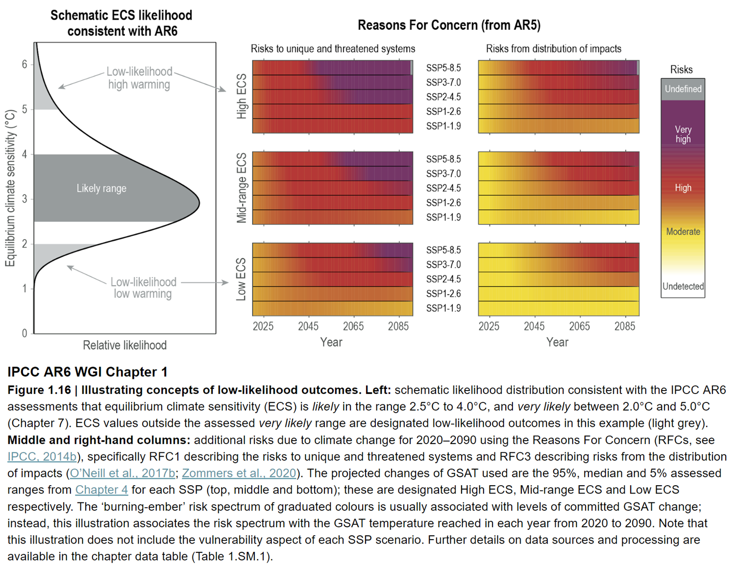
Fig. 1: Left: schematic likelihood distribution consistent with the IPCC AR6 assessments that equilibrium climate sensitivity (ECS) is likely in the range 2.5°C to 4.0°C, and very likely between 2.0°C and 5.0°C. ECS values outside the assessed very likely range are designated low-likelihood outcomes in this example (light grey). Middle and right-hand columns: additional risks due to climate change for 2020 to 2090. Source: IPCC AR6 WGI Chapter 6 Figure 1-16.
It’s all a matter of degree
All the models and evidence confirm a minimum warming close to 2°C for a doubling of atmospheric CO2 with a most likely value of 3°C and the potential to warm 4°C or even more. These are not small rises: they would signal many damaging and highly disruptive changes to the environment (fig. 1). In this light, the arguments against reducing greenhouse gas emissions because of "low" climate sensitivity are a form of gambling. A minority claim the climate is less sensitive than we think, the implication being that as a consequence, we don’t need to do anything much about it. Others suggest that because we can't tell for sure, we should wait and see. Both such stances are nothing short of stupid. Inaction or complacency in the face of the evidence outlined above severely heightens risk. It is gambling with the entire future ecology of the planet and the welfare of everyone on it, on the rapidly diminishing off-chance of being right.
Last updated on 12 November 2023 by John Mason. View Archives


Klapper... The Smith etal paper that Tom links to bears reviewing, especially the summary and conclusions. This sums up some of the things I've been attempting to state with regards to the relationship between observations and models, where I've said that it's reasonable to conclude that the models are better representing the climate system and our observations are challenge our ability to "close the Earth's energy budget."
What I see you doing (or at least believe I see you doing) is getting stuck in down in the weeds of our observations, assuming they have to be somehow correct. I think that's a misdirected approach. As I've said several times in our conversation so far, there are lots of uncertainties in the empirical evidence and the models are there to contrain those uncertainties.
Klapper - It is wholly unreasonable to discard ocean heat content data prior to 2005. While the XBT data has higher uncertainties than ARGO, and there have been several calibration issues with it that are recently resolved, the sampling back to the 1960's is more than sufficient to establish long term growth in ocean heat content. There simply isn't enough deviation in temperature anomalies over distance to reject long term warming of about 0.6C/decade even with sparse XBT sampling.
For details on this, including evaluating the standard deviation of anomalies against distance, see the Levitus et al 2012, specifically the "Appendix: Error Estimates of Objectively Analyzed Oceanographic Data", which speaks directly to this matter. The uncertainty bounds from Levitus et al are shown in Fig. 2 here. And they are certainly tight enough to establish warming.
@Rob Honeycutt #326:
"...assuming they have to be somehow correct..."
Oh I don't assume they have to be correct at all. You can take the Net observations (satellite) from the Smith paper and throw them in the trashcan. However, that's not true of the ARGO data. Our knowledge of ocean heat is much much better since 2005 or 2004 than pre 2005 or 2004.
@KR #327:
The problem is the XBT data only go down to 700 m. If I had tried to use only 0-700 heat gain as my metric, I would be jumped on big time since I was "ignoring" the deeper ocean. The amount of sampling below 700 m prior to the ARGO network is extremely sparse, as noted in the Smith et al paper, particularly in the southern ocean.
@Tom Curtis #322:
"...That Klapper is still using it shows he is clinging to old data simply because it is convenient for his message..."
Absolutely not true (and an unecessary cheap shot to boot). I extracted the multi-run per model ensemble mean numbers from KNMI data explorer, CMIP5 rpc4.5 scenario. I also checked one individual run from the GISS EH2 model, same emissions scenario (although it makes no real difference between the scenarios in the 2005 to 2015 period).
I used the rlut, rsdt, and rsut variables (absolute values, not anomalies) to calculate my net. I'm looking into the difference between my Net TOA imbalance and Smith et al, but not tonight.
Klapper - The XBT data does go to (and through) 2000 meters. Yes, XBT data back to the 1950's is sparse below 700 meters, but it is still data, and uncertainties due to sparse sampling are considerably smaller than the ocean heat content trends over the time of observations.
Again, I would refer you to Levitus et al 2012, in particular Fig. 1 and the supplemental figure S10, which shows the 0-2000m 2-sigma uncertainties, variances, and trends for each ocean basin. We have enough data to establish long term OHC trends with some accuracy.
Klapper - My apologies, S10 in Levitus et al is for the thermosteric component, while S1 shows the OHC (1022 J). Again, there is sufficient data to establish a long term trend against sampling uncertainties 0-2000m.
Klapper @328... Just to trying to simplify things here, so your key issue is that measured changes in OHC data (W/m^2) do not match model results for TOA imbalance.
Given the preceding thread at the Guardian prior to the start here at SKS, was a thread discussion beginning here and running to 7,000 words of comment with nothing resolved, I would suggest a little discipline is required here at SKS to prevent it becoming another pantomime.
The issue to hand is "the missing 0.5W/m2 between models and reality." Such a quantity was identified @322 as having been "based on old figures from CMIP 4 and far less accurate observations, and even then is exaggerated by rounding."
This is refuted @330 as being "absolutely not true" because the missing 0.5W/m2 is apparently a different 0.5W/m2 to that identified @322, and for which we await a full description.
Looking back at the Guardian thread, the 0.5W/m2 appears here as the difference between study-based "heat gain in the measurable part of the ocean .. in the range of 0.3 to 0.6 W/m2" yielding a "best guess at ocean heat gain (of) 0.5W/m2" and "Models show(ing) the imbalance at the top of the atmosphere through this period as being 1.0 W/m2."
So what period? What models? Is the TOA 1.0 W/m2 anything to do with the "TOA energy imbalance projections from the models (of) ... currently about 1.0 to 1.2 W/m2" mentioned in the Guardian thread here?
Please let us not spend many thousands more words without a grip on what is being discussed.
Klapper - you are proposing to ignore OHC pre-Argo because there is only data to 700m. However, if you wish to postulate that the huge change in OHC 0-700m does not mean energy imbalance, then you must also be proposing that there could somehow cooling of the 700-2000 layer to compensate for warming in the upper layer.
I would also be interested in your opinion on the Loeb et al 2012 paper in claiming that models and observations are at odds.
Scaddenp - We do have XBT data below 700m, just rather less of it. Which is how the ocean heat content analyses going back to the 1950s have been done.
@MA Rodger #334:
To cross-check my model vs actual comparison for TOA energy imbalance I extracted at the KNMI Data Explorer site data from the CMIP5 Model Ensemble RCP 4.5 (all runs) the variables rsut, rlut, and rsdt, monthly data. I averaged the monthly global data into annual global numbers and calculated the TOA energy imbalance per year as rlut + rsut - rsdt.
To compare to a published number, in this case I'll use the Hansen et al number from the GISS website linked above, I averaged the years from my model extraction data, in this case 2005 to 2010. The GISS number for global TOA energy imbalance of 0.58 W/m2 +/- 0.15. This agrees with other published estimates of similar time periods.
The average I get from my CMIP5 RCP 4.5 ensemble annual data, 2005 to 2010 inclusive is 0.92 W/m2. The models appeart to be running too hot by a substantial amount.
My next experiment will be to compare these TOA CMIP5 data to OHC over a longer period, say 2000 to 2014 inclusive. Or maybe just OHC from 2005 to 2014 since the ARGO spatial density was essentially full coverage after 2004 or 2005. We can likely agree that the global energy imbalance dominantly present in the ocean heat gain, although some of the imbalance goes into the atmosphere and melting continental ice.
Klapper - 5 to (at most) 15 year periods are short enough that statistical significance is lacking, and that the model mean is expected to differ from short term variations such as ENSO.
I don't think you can make any significant conclusions from such a short period of data.
Klapper/everyone - I'll note that many of Klappers issues with model fidelity have been discussed at great length over on the Climate Models show remarkable agreement with recent surface warming thread. And on that thread Klapper was shown (IMO) that his arguments did not hold.
This appears to be yet another search for a (notably short term, and hence statistically insignificant) criteria with which to dismiss modeling.
Klapper @337:
1) Did you compute (∑rlut x 1/n) + (∑rsut x 1/n) - (∑rsdt x 1/n) or (∑(rlut + rsut - rsdt)) x 1/n?
2) The IPCC uses just one model run per model in calculating multi-model means for a reason. Failing to do so allows a few models with unusually large numbers of runs to be more heavilly weighted in the absence of evidence that those models are superior, and indeed, regardless of any evidence of their superiority or inferiority. In particular, one model with multiple runs is the GISS model ER, which you have previously stated has a TOA energy imbalance from 2000-2015 of 1.2 W/m^2 - ie, it is at the high end of the CMIP 5 range, and above the CMIP 5 multi-run mean as calculated by you. There is reason to think this distorts your result.
3) 5 years is too short a time for such comparisons for reasons given by KR. What are your results for 2000-2010 for comparison with the Smith et al data? Indeed, what are your results for all of the Smith et al periods as shown in the second panel of the first graph in my post @322?
4) Why do you use the multi-model (really multi-run) mean rather than the multi-model median as do Smith et al? In this case where damage functions are not a factor, using the median as the central estimate makes sense (IMO) in that it is less subject to distortion by outliers. Is their some reason why you preffer it despite this disadvantage?
5) I ask you to forgive me for not responding to your earlier posts. I had an extensive response prepared and lost it in the attempt to post it. Unfortunately I have been ill since then, and not had the energy for recomposing a similarly extensive response. I am also considering whether or not to download the data from KNMI for direct comparison before more detailed response (which will take more energy and concentration).
Klapper @337.
You are getting your 0.58 W/m2 +/- 0.15 from Hansen et al (2012) , a paper which states:-
I would suggest that such a quote is difficult to ignore, although you apparently do overlook it. It sort-of adds weight to the comment by KR @338. From memory, the negative solar forcing through those years between cycle 23 & 24 was something like -0.13W/m2, reducing your mismatch from the range 0.19-0.49 W/m2 to 0.06-0.36 W/m/2, considerably reduced from the originally stated 0.5 W/m2.
The paper goes on to say:-
Again, here is very relevant data you overlook. If these AR4 models underestimate negative aerosol forcing, you would expect them to run with a greater TOA imbalance. And if they did so in AR4, would more recent models be expected now to conform to Hansen et al (2012)? Or is that a bit of an assumption on your part?
@KR #338:
"I don't think you can make any significant conclusions from such a short period of data".
The quality data for OHC only begin since the ARGO system reached a reasonable spatial density (say 2004 at the earliest). However I will look for some longer OHC/global heat gain data/estimates to match longer periods, say a 15 year period from 2000 to 2014 inclusive. The average for that period is a TOA energy imbalance of 0.98W/m2 from the CMIP5 ensemble (multi-runs per model) mean rcp4.5 scenario.
@Tom Curtis #340:
"..The IPCC uses just one model run per model in calculating multi-model means for a reason."
Yes very egalitarian of them. An argument could be made for using the other ensemble which says, the better resource supported models have more runs and are probably more realistic than the less resourced models. However, it doesn't make much difference, as the 2005 to 2010 average TOA imbalance changes from 0.92 to 0.90W/m2 with the one run per model ensemble.
"..What are your results for 2000-2010 for comparison with the Smith et al data?"
The 2000 to 2010 average TOA energy imbalance is +0.95W/m2.
".. rather than the multi-model median as do Smith et al?"
I would have to download all the models, a very tedious process, and create my own median; KNMI only options a mean in their ensemble exports.
@MA Rodger #341:
".. reducing your mismatch from the range 0.19-0.49 W/m2 to 0.06-0.36 W/m/2, considerably reduced from the originally stated 0.5 W/m2"
You're forgetting the originally stated comparison was to OHC, not global energy imbalance (although as noted OHC pretty much is the bulk of the energy imbalance). In any case, even reduced, the numbers support my hypothesis the models run too hot.
"..implies that the aerosol forcing is about -1.6 W/m2"
Circular logic but that's a topic for whole discussion on itself. I'll say no more.
"..would more recent models be expected now to conform to Hansen et al (2012)?"
I'm using the more recent models (CMIP5) and they don't conform to Hansen et al 2012 (still too hot). I'm tempted to go get the AR4 model ensemble and try that also, but for now I'm off to work.
Klapper @343:
1) I need to make a correction. I assumed that Smith et al presented a median value based on their use of a box plot. In their supplementary information, however, they describe the central value as a mean, and the "first quartile" and "third quartile" values as being minus and plus one standard deviation respectively, with whiskers showing the range. The values are given as 0.73 +/- 0.13 W/m^2 with a range from 0.43 - 0.97 W/m^2. These values are stated as being the anomaly values with respect to the preindustrial era - anomaly values being used as a correction for model drift.
2) As noted before, the difference between observations and models over this period in Smith et al is 0.11 W/m^2. Even using your uncorrected values, the difference between observed and modelled TOA energy imbalance from 2000-2010 is still only 0.33 W/m^2. The +/- 2 sigma range of the observed TOA energy imbalance is 0.06 to 1.18 W/m^2. So, even on your figures the discrepancy between mean model and mean observed TOA energy imbalance is substantially less than 0.5 W/m^2 (which as I said before, is a fiction). Further, you are making a case that the models are shown to be seriously flawed because, the modelled TOA energy imbalance lies within error (actually, withing 1.2 SDs) of the observed value. It may make a good emotive argument, but it is certainly not a scientific argument.
Klapper - We have OHC data of reasonable quality back to the 1960s, as I noted here. What you are considering is far too short a period for statistical significance, hence too short to make broad statements about model fidelity. If you want to make any claims regarding the differences I would suggest using a sufficient amount of the available data.
You're arguing about short term unforced variations, not statistically significant long term climate trends, and your complaints about the XBT data don't change that fact.
Might suggest to one and all that this conversation about model fidelity shift to the appropriate thread on climate models?
@Tom Curtis #345:
"..So, even on your figures the discrepancy between mean model and mean observed TOA energy imbalance is substantially less than 0.5 W/m^2 (which as I said before, is a fiction)".
You're ignoring my comment above in which I clearly stated the 0.5 W/m2 was the difference between OHC and the TOA model output. Here's my 2 most succinct posts from the Guardian on the source of the 0.5 W/m2 number:
"All that being said, these studies would agree the heat gain in the measurable part of the ocean is in the range of 0.3 to 0.6 W/m2. If the best guess at ocean heat gain is 0.5W/m2, then where is the rest of the heat? Models show the imbalance at the top of the atmosphere through this period as being 1.0 W/m2. We know the atmosphere has limited heat capacity, and the troposphere hasn't shown significant warming since 2005 in any case. That leaves ice melting."
"However, heat gain by the oceans right now might be 0.5W/m2, which is only 1/2 of the projected TOA energy imbalance, so while the oceans are warming, and the atmosphere very weakly so, together they don't account for the model predicted 1.0 to 1.2 W/m2 TOA net energy input."
I concede in at least one post I used the OHC delta to TOA model as "shorthand" for the global energy delta to model TOA, but it's clear from my initial posts the source of the numbers. You're either not reading my full posts or you're deliberately ignoring the context.
@Tom Curtis #345:
"...anomaly values being used as a correction for model drift."
Why don't you expand on what you think is going on here. I'm using the absolute numbers from the mean CMIP5 ensemble, which I think is the correct thing to do. What do you (and Smith et al) mean by "model drift"?
@KR #347:
"...We have OHC data of reasonable quality back to the 1960s"
I've looked at the quarterly/annual sampling maps for pre-Argo at various depths and I wouldn't agree that's true for 0-700 m depth and certainly not true for 0-2000 m. There's a reason Lyman & Johnson 2014 (and other stuides) don't calculate heat changes prior to 2004 for depths greater than 700 m; they are not very meaningful.