


 Arguments


Are surface temperature records reliable?
What the science says...
| Select a level... |
 Basic
Basic
|
 Intermediate
|
 Advanced
| ||||
|
The warming trend is the same in rural and urban areas, measured by thermometers and satellites, and by natural thermometers. |
|||||||
Climate Myth...
Temp record is unreliable
"We found [U.S. weather] stations located next to the exhaust fans of air conditioning units, surrounded by asphalt parking lots and roads, on blistering-hot rooftops, and near sidewalks and buildings that absorb and radiate heat. We found 68 stations located at wastewater treatment plants, where the process of waste digestion causes temperatures to be higher than in surrounding areas.
In fact, we found that 89 percent of the stations – nearly 9 of every 10 – fail to meet the National Weather Service’s own siting requirements that stations must be 30 meters (about 100 feet) or more away from an artificial heating or radiating/reflecting heat source." (Watts 2009)
At a glance
It's important to understand one thing above all: the vast majority of climate change denialism does not occur in the world of science, but on the internet. Specifically in the blog-world: anyone can blog or have a social media account and say whatever they want to say. And they do. We all saw plenty of that during the Covid-19 pandemic, seemingly offering an open invitation to step up and proclaim, "I know better than all those scientists!"
A few years ago in the USA, an online project was launched with its participants taking photos of some American weather stations. The idea behind it was to draw attention to stations thought to be badly-sited for the purpose of recording temperature. The logic behind this, they thought, was that if temperature records from a number of U.S. sites could be discredited, then global warming could be declared a hoax. Never mind that the U.S. is a relatively small portion of the Earth;s surface. And what about all the other indicators pointing firmly at warming? Huge reductions in sea ice, poleward migrations of many species, retreating glaciers, rising seas - that sort of thing. None of these things apparently mattered if part of the picture could be shown to be flawed.
But they forgot one thing. Professional climate scientists already knew a great deal about things that can cause outliers in temperature datasets. One example will suffice. When compiling temperature records, NASA's Goddard Institute for Space Studies goes to great pains to remove any possible influence from things like the urban heat island effect. That effect describes the fact that densely built-up parts of cities are likely to be a bit warmer due to all of that human activity.
How they do this is to take the urban temperature trends and compare them to the rural trends of the surrounding countryside. They then adjust the urban trend so it matches the rural trend – thereby removing that urban effect. This is not 'tampering' with data: it's a tried and tested method of removing local outliers from regional trends to get more realistic results.
As this methodology was being developed, some findings were surprising at first glance. Often, excess urban warming was small in amount. Even more surprisingly, a significant number of urban trends were cooler relative to their country surroundings. But that's because weather stations are often sited in relatively cool areas within a city, such as parks.
Finally, there have been independent analyses of global temperature datasets that had very similar results to NASA. 'Berkeley Earth Surface Temperatures' study (BEST) is a well-known example and was carried out at the University of California, starting in 2010. The physicist who initiated that study was formerly a climate change skeptic. Not so much now!
Please use this form to provide feedback about this new "At a glance" section, which was updated on May 27, 2023 to improve its readability. Read a more technical version below or dig deeper via the tabs above!
Further details
Temperature data are essential for predicting the weather and recording climate trends. So organisations like the U.S. National Weather Service, and indeed every national weather service around the world, require temperatures to be measured as accurately as possible. To understand climate change we also need to be sure we can trust historical measurements.
Surface temperature measurements are collected from more than 30,000 stations around the world (Rennie et al. 2014). About 7000 of these have long, consistent monthly records. As technology gets better, stations are updated with newer equipment. When equipment is updated or stations are moved, the new data is compared to the old record to be sure measurements are consistent over time.
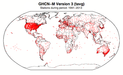
Figure 1. Station locations with at least 1 month of data in the monthly Global Historical Climatology Network (GHCN-M). This set of 7280 stations are used in the global land surface databank. (Rennie et al. 2014)
In 2009 allegations were made in the blogosphere that weather stations placed in what some thought to be 'poor' locations could make the temperature record unreliable (and therefore, in certain minds, global warming would be shown to be a flawed concept). Scientists at the National Climatic Data Center took those allegations very seriously. They undertook a careful study of the possible problem and published the results in 2010. The paper, "On the reliability of the U.S. surface temperature record" (Menne et al. 2010), had an interesting conclusion. The temperatures from stations that the self-appointed critics claimed were "poorly sited" actually showed slightly cooler maximum daily temperatures compared to the average.
Around the same time, a physicist who was originally hostile to the concept of anthropogenic global warming, Dr. Richard Muller, decided to do his own temperature analysis. This proposal was loudly cheered in certain sections of the blogosphere where it was assumed the work would, wait for it, disprove global warming.
To undertake the work, Muller organized a group called Berkeley Earth to do an independent study (Berkeley Earth Surface Temperature study or BEST) of the temperature record. They specifically wanted to answer the question, “is the temperature rise on land improperly affected by the four key biases (station quality, homogenization, urban heat island, and station selection)?" The BEST project had the goal of merging all of the world’s temperature data sets into a common data set. It was a huge challenge.
Their eventual conclusions, after much hard analytical toil, were as follows:
1) The accuracy of the land surface temperature record was confirmed;
2) The BEST study used more data than previous studies but came to essentially the same conclusion;
3) The influence of the urban stations on the global record is very small and, if present at all, is biased on the cool side.
Muller commented: “I was not expecting this, but as a scientist, I feel it is my duty to let the evidence change my mind.” On that, certain parts of the blogosphere went into a state of meltdown. The lesson to be learned from such goings on is, “be careful what you wish for”. Presuming that improving temperature records will remove or significantly lower the global warming signal is not the wisest of things to do.
The BEST conclusions about the urban heat effect were nicely explained by our late colleague, Andy Skuce, in a post here at Skeptical Science in 2011. Figure 2 shows BEST plotted against several other major global temperature datasets. There may be some disagreement between individual datasets, especially towards the start of the record in the 19th Century, but the trends are all unequivocally the same.
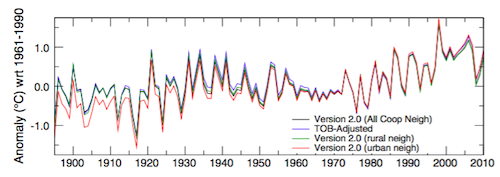
Figure 2. Comparison of spatially gridded minimum temperatures for U.S. Historical Climatology Network (USHCN) data adjusted for time-of-day (TOB) only, and selected for rural or urban neighborhoods after homogenization to remove biases. (Hausfather et al. 2013)
Finally, temperatures measured on land are only one part of understanding the climate. We track many indicators of climate change to get the big picture. All indicators point to the same conclusion: the global temperature is increasing.
See also
Understanding adjustments to temperature data, Zeke Hausfather
Explainer: How data adjustments affect global temperature records, Zeke Hausfather
Time-of-observation Bias, John Hartz
Check original data
All the Berkeley Earth data and analyses are available online at http://berkeleyearth.org/data/.
Plot your own temperature trends with Kevin's calculator.
Or plot the differences with rural, urban, or selected regions with another calculator by Kevin.
NASA GISS Surface Temperature Analysis (GISSTEMP) describes how NASA handles the urban heat effect and links to current data.
NOAA Global Historical Climate Network (GHCN) Daily. GHCN-Daily contains records from over 100,000 stations in 180 countries and territories.
Last updated on 27 May 2023 by John Mason. View Archives


- unified documentation of the procedure, including scientific justification and specification of algorithms applied is not available
- for step 2, 3, 4 & 6 at least references to papers are provided, for step 5 not even that
- neither executables nor source code and program documentation is provided for programs TOBS, MMTS, SHAP & FILNET.
- metadata used by the programs above to do their job is missing and/or unspecified
- clear statement whether the same automatic procedure were applied to GHCN v2 which is hinted at the USHCN Version 1 site is missing (if the arcane wording "GHCN Global Gridded Data" in the HTML header of that page is dismissed)
Well, I have found something, not referenced in either USHCN or GHCN pages. It is ftp://ftp.ncdc.noaa.gov/pub/data/ushcn/v2/monthly/software/USHCN_v52d.20100217.tar.gz. There is software there (written in Fortran 77) and some rather messy documentation including an MS Word DOC file titled: I do not know how authoritative it is. But I do know much better documentation is needed even on low budget projects, not to mention one multi thousand billion bucks policy decisions are supposed to be based on. The "Pairwise Homogeneity Algorithm (PHA)" promoted (but not specified) in this document is not referenced on any other USHCN or GHCN page. Google search "Pairwise Homogeneity Algorithm" site:gov returns empty. It would be a major job to do the usual software audit on this thing. One has to hire & pay people with the right expertise for it, then publish the report along with data. However, any scientist would run away screaming upon seeing a calibration curve like this, wouldn't she? It is V shaped with clear trends and multiple step-like changes. One would think with 6736 stations spread all over the world and 176 years in time providing 4,864,014 individual data points errors would be a little bit more independent allowing for the central limit theorem to kick in. At least some very detailed explanation is needed why are there unmistakable trends in adjustments commensurate with the effect to be uncovered and why this trend has a steep downward slope for the first half of epoch while just the opposite is true for the second half? BTW, the situation with USHCN is a little bit worse. Adjustment for 1934 is -0.465°C relative to those applied to 2007-2010 (like 0.6°C/century?). I'll post the USHCN graph later. #66 scaddenp at 12:39 PM on 29 June, 2010 you think that you can explain warming in ocean, satellite, and surface record away as "anomalies" as poor instrumental records, and then explain the loss of ice/snow around the world purely by black soot? And the sealevel rise as by soot-induced melting alone without thermal expansion? I guess similar strange measurement anomalies will explain upper stratospheric cooling and the IR spectrum changes at TOS and at surface. That is drawing one very long bow One thing at a time, please. Let's focus on the problem at hand first, the rest can wait.[Oops. Pressed the wrong button first] $ wget ftp://ftp.ncdc.noaa.gov/pub/data/ghcn/v2/v2.mean* $ grep '^425' v2.mean > ushcn.mean $ grep '^425' v2.mean_adj > ushcn.adj $ cat ushcn.mean|perl -e 'while (<>) {chomp; $id=substr($_,0,12); $y=substr($_,12,4); for ($m=1;$m<=12;$m++) {$t=substr($_,11+5*$m,5); printf "%s_%s_%02u %5d\n",$id,$y,$m,$t;} }'|grep -v ' [-]9999$' > ushcn.mean_monthly $ cat ushcn.adj|perl -e 'while (<>) {chomp; $id=substr($_,0,12); $y=substr($_,12,4); for ($m=1;$m<=12;$m++) {$t=substr($_,11+5*$m,5); printf "%s_%s_%02u %5d\n",$id,$y,$m,$t;} }'|grep -v ' [-]9999$' > ushcn.adj_monthly $ cut -c-20 ushcn.mean_monthly | sort > ushcn.mean_monthly_id $ cut -c-20 ushcn.adj_monthly | sort > ushcn.adj_monthly_id $ uniq -d ushcn.mean_monthly_id $ uniq -d ushcn.adj_monthly_id $ sort ushcn.mean_monthly_id ushcn.adj_monthly_id | uniq -d > ushcn.common_monthly_id $ (sed -e 's/^/0 /g' ushcn.mean_monthly; sed -e 's/^/1 /g' ushcn.adj_monthly; sed -e 's/^/2 /g' ushcn.common_monthly_id;)|sort +1 -2 +0 -1 > ushcn.composite_list $ sed -e 's/ */ /g' ushcn.composite_list|perl -e 'while (<>) {chomp; ($i,$id,$t)=split; if ($i==2 && $id eq $iid && $id eq $iiid) {$d=$tt-$ttt; printf "%s %d\n",$id,$d;} $iiid=$iid; $iid=$id; $ttt=$tt; $tt=$t;}' > ushcn.adjustments_monthly_by_station $ sed -e 's/^............_//g' -e 's/_.. / /g' ushcn.adjustments_monthly_by_station | sort > ushcn.adjustments_annual_list $ echo '#' >> ushcn.adjustments_annual_list $ cat ushcn.adjustments_annual_list | perl -e 'while (<>) {chomp; ($d,$t)=split; if ($d ne $dd && $dd ne "") {$x/=$n*10; printf "%s\t%.3f\n",$dd,$x; $n=0; $x=0;} $n++; $x+=$t; $dd=$d;}' > ushcn.adjustments_annual.txt $ openoffice -calc ushcn.adjustments_annual.txt